A Note on Surface Integrals

In this post, we will prove a useful theorem about surface integrals. The theorem is simple to conceptualize, but difficult to state precisely. The idea is that we can compute a surface integral for any surface embedded in \(\mathbb{R}^3\) entirely in terms of the maximal component of the unit normal vector at each point along the surface. Consider the following illustration:

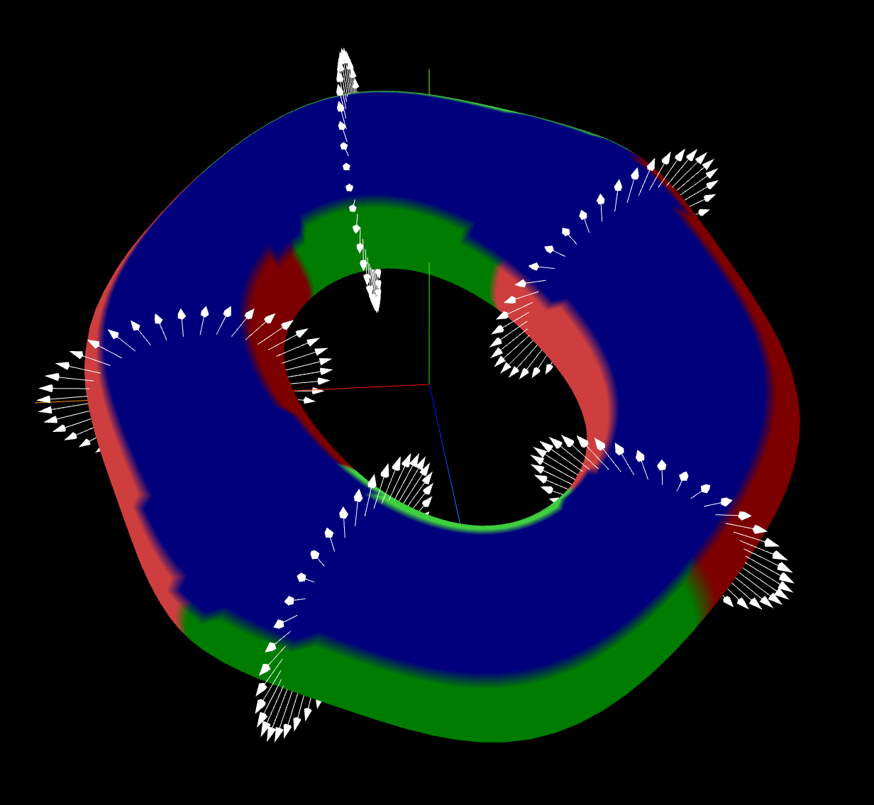
The idea is to systematically determine a set of parameterizations of an arbitrary surface based solely on the unit normal vector field along the surface. The set of points where the the maximal component of the unit normal vector field is uniform comprise an open set, i.e. a "patch" of the surface, and these patches cover the surface except for their "seams" (which are piecewise curves), so their closures cover the surface. We can then project each of these patches onto a coordinate domain in \(\mathbb{R}^2\) to determine domains of integration. The Implicit Function Theorem ensures that there is some parameterization that maps from the closure of each domain to the respective patch. Together, these parameterizations parameterize the entire surface. We can then use them to compute surface integrals, in particular, we can use them to compute the area of the surface.

Here is the precise statement of the theorem:

Theorem. Let \(S\) be any compact oriented smooth \(2\)-manifold embedded in \(\mathbb{R}^3\) and \(N\) be any smooth unit normal vector field along \(S\) consistent with the orientation of \(S\). Then

\[\mathrm{Area}(S) = \int_S~dS = \sum_{\alpha \in \mathcal{A}}\int_{D_{\alpha}}\frac{1}{\lvert N_{c(\alpha)} \circ F_{\alpha}\rvert}~dA_{\alpha},\]

where \(dS\) is the volume form,

\[\mathcal{A} = \{(x, +1, y, z), (x, -1, y, z), (y, +1, z, x), (y, -1, z, x), (z, +1, x, y), (z, -1, x, y)\},\]

\((x,y,z)\) are the standard coordinate functions on \(\mathbb{R}^3\), the functions \(c, s, c_1, c_2\) are defined such that

\[\alpha = (c(\alpha), s(\alpha), c_1(\alpha), c_2(\alpha)),\]

the sets \(D_{\alpha}\) are defined as

\[D_{\alpha} = \pi_{\alpha}(W_{\alpha})\]

where \(\pi_{\alpha} : S \rightarrow \mathbb{R}^2\) is the projection

\[\pi_{\alpha}(p) = (c_1(\alpha)(p), c_2(\alpha)(p)),\]

and

\[W_{\alpha} = \{p \in S \mid s(\alpha) \cdot N(p)_{c(\alpha)} \gt \lvert N(p)_{c_1(\alpha)}\rvert \text{ and } s(\alpha) \cdot N(p)_{c(\alpha)} \gt \lvert N(p)_{c_2(\alpha)}\rvert\},\]

and the functions \(F_{\alpha} : \overline{D_{\alpha}} \rightarrow W_{\alpha}\) are certain smooth maps that restrict to diffeomorphisms from \(D_{\alpha}\) onto \(W_{\alpha}\) and the differential forms \(A_{\alpha}\) are defined as

\[A_{\alpha} = d(c_1(\alpha)) \wedge d(c_2(\alpha)).\]

Preliminaries

First, we recall some general definitions and theorems related to surface integrals.

Definition (Domain of Integration). A domain of integration is a subset \(D \subseteq \mathbb{R}^n\) such that \(D\) is bounded and \(\partial D\) has \(n\)-dimensional measure \(0\).

We invoke the following two theorems (quoted from the book Introduction to Smooth Manifolds by John Lee):

Theorem (Integration by Parameterizations) [Lee]. Let \(M\) be an oriented, smooth \(n\)-manifold with or without boundary, and let \(\omega\) be a compactly-supported \(n\)-form on \(M\). Suppose \(D_1, \dots, D_k\) are open domains of integration in \(\mathbb{R}^n\) and, for \(i = 1,\dots,k\), we are given smooth maps \(F_i : \bar{D_i} \rightarrow M\) satisfying the following conditions:

• \(F_i\) restricts to an orientation-preserving diffeomorphism from \(D_i\) onto an open subset \(W_i \subseteq M\);
• \(W_i \cap W_j = \emptyset\) when \(i \ne j\);
• \(\mathrm{supp}(\omega) \subseteq \bar{W_1} \cup \dots \cup \bar{W_k}\);

Then

\[\int_M \omega = \sum_{i=1}^k \int_{D_i} F_i^*\omega.\]

Theorem (Volume Forms via Normals) [Lee]. Let \((M,g)\) be an oriented Riemannian manifold with or without boundary, let \(S \subseteq M\) is an immersed hypersurface with or without boundary, and let \(\overline{g}\) denote the induced metric on \(S\). Suppose \(N\) is a smooth unit normal vector field along \(S\). With respect to the orientation of \(S\) determined by \(N\), the volume form of \(S, \overline{g}\) is given by

\[\omega_{\overline{g}} = \iota_S^*(N \lrcorner \omega_g),\]

where \(\iota : S \rightarrow M\) is the injection, and \(\omega_g\) is the volume form corresponding to the metric \(g\).

The Proof of the Theorem

We seek to find a suitable set of parameterizations for an arbitrary surface.

Let \(S \subseteq \mathbb{R}^3\) denote an arbitrary compact oriented embedded smooth \(2\)-manifold. Let \((x,y,z)\) denote the standard coordinates on \(\mathbb{R}^3\), namely, the component functions of the identity map \(\mathrm{id} : \mathbb{R}^3 \rightarrow \mathbb{R}^3\). Let \(g = dx^2 + dy^2 + dz^2\) denote the Euclidean metric on \(\mathbb{R}^3\). Every normal vector field \(N\) may be expressed in standard coordinates as

\[N = N_x \cdot \frac{\partial}{\partial x} + N_y \cdot \frac{\partial}{\partial y} + N_z \cdot \frac{\partial}{\partial z},\]

and every normal vector \(N_p\) along this field may be expressed in standard coordinates as

\[N_p = N_x(p) \cdot \frac{\partial}{\partial x}\bigg\rvert_p + N_y(p) \cdot \frac{\partial}{\partial y}\bigg\rvert_p + N_z(p) \cdot \frac{\partial}{\partial z}\bigg\rvert_p.\]

Every unit normal vector satisfies \(\langle N_p, N_p \rangle_{g_p} = 1\), which implies that, in coordinates,

\[N_x(p)^2 + N_y(p)^2 + N_z(p)^2 = 1.\]

We define the following open subsets of \(S\):

• \(W_x^+ = \{p \in S \mid N_x(p) \gt \lvert N_y(p) \rvert \text{ and } N_x(p) \gt \lvert N_z(p) \rvert\}\),
• \(W_x^- = \{p \in S \mid -N_x(p) \gt \lvert N_y(p) \rvert \text{ and } -N_x(p) \gt \lvert N_z(p) \rvert\}\),
• \(W_y^+ = \{p \in S \mid N_y(p) \gt \lvert N_x(p) \rvert \text{ and } N_y(p) \gt \lvert N_z(p) \rvert\}\),
• \(W_y^- = \{p \in S \mid -N_y(p) \gt \lvert N_x(p) \rvert \text{ and } -N_y(p) \gt \lvert N_z(p) \rvert\}\),
• \(W_z^+ = \{p \in S \mid N_z(p) \gt \lvert N_x(p) \rvert \text{ and } N_z(p) \gt \lvert N_y(p) \rvert\}\),
• \(W_z^- = \{p \in S \mid -N_z(p) \gt \lvert N_x(p) \rvert \text{ and } -N_z(p) \gt \lvert N_y(p) \rvert\}\).

We will show that \(W_z^+\) is an open set. Define the functions \(f_1, f_2 : S \rightarrow \mathbb{R}\) as follows:

• \(f_1(p) = N_z(p) - \lvert N_x(p) \rvert\),
• \(f_2(p) = N_z(p) - \lvert N_y(p) \rvert\).

Since \(N\) is smooth, each component function \(N_x, N_y, N_z\) is smooth and hence continuous. Thus, \(f_1\) and \(f_2\) are continuous. The set of points where \(N_z(p) \gt \lvert N_x(p) \rvert\) is precisely \(f_1^{-1}(0, \infty)\), which is open since it is the pre-image of an open set under a continuous function. The set of points where \(N_z(p) \gt \lvert N_y(p) \rvert\) is precisely \(f_2^{-1}(0, \infty)\), which is open since it is the pre-image of an open set under a continuous function. Thus, \(W_z^+ = f_1^{-1}(0, \infty) \cap f_2^{-1}(0, \infty)\) is open since it is the intersection of open sets.

Next, we show that these sets are pairwise disjoint. Consider the example of \(W_x^+\) and \(W_y^+\). If \(p \in W_x^+ \cap W_y^+\), then \(N_x(p) \gt \lvert N_y(p) \rvert\) and \(N_y(p) \gt \lvert N_x(p) \rvert\), which implies that \(N_x(p) \gt N_x(p)\), a contradiction. Thus, these sets are pairwise disjoint.

Next, note that the closures of these sets cover \(S\). Let \(p \in S\). Suppose that there is some maximal component of the unit normal vector \(N_p\), e.g., \(N_z(p)\). Then \(p \in W_z^+\) by definition. If there is a "tie", e.g., \(\lvert N_z(p) \rvert = \lvert N_x(p) \rvert\), then \(p\) will lie in the boundary of one of the sets and hence in its closure. Thus, these sets cover \(S\), and since \(\mathrm{supp}(dS) \subseteq S\), the union of these sets contains the support of \(dS\).

Next, we define the following projection maps with signature \(S \rightarrow \mathbb{R}^2\):

• \(\pi_x(x,y,z)= (y,z)\),
• \(\pi_y(x,y,z) = (x,z)\),
• \(\pi_z(x,y,z) = (x,y)\).

We then define the following sets in \(\mathbb{R}^2\):

• \(D_x^+ = \pi_x(W_x^+)\),
• \(D_x^- = \pi_x(W_x^-)\),
• \(D_y^+ = \pi_y(W_y^+)\),
• \(D_y^- = \pi_y(W_y^-)\),
• \(D_z^+ = \pi_z(W_z^+)\),
• \(D_z^- = \pi_z(W_z^-)\).

We will show that \(D_z^+\) is bounded. The projection map \(\pi_z\) is continuous. Since \(W_z^+\) is open, \(\overline{W_z^+}\) is closed. Since \(\overline{W_z^+} \subset S\) and \(S\) is compact, \(\overline{W_z^+}\) is compact. Thus, since \(\pi_z\) is continuous, \(\pi_z(W_z^+)\) is compact. By the Heine-Borel Theorem, every compact subset of \(\mathbb{R}^2\) is bounded. Thus, \(D_z^+ = \pi_z(W_z^+) \subseteq \pi_z(\overline{W_z^+})\) is bounded.

Next, we will show that \(D_z^+\) is open. The projection map \(\pi_z : \mathbb{R}^3 \rightarrow \mathbb{R}^2\) is a linear map. The differential \(d(\pi_z)_p : T_p\mathbb{R}^3 \rightarrow T_{\pi_z(p)}\mathbb{R}^2\) is also a linear map, and is precisely the map

\[d(\pi_z)_p\left(x \cdot \frac{\partial}{\partial x}\bigg\vert_p + y \cdot \frac{\partial}{\partial y}\bigg\vert_p + z \cdot \frac{\partial}{\partial z}\bigg\vert_p\right) = x \cdot \frac{\partial}{\partial x}\bigg\vert_p + y \cdot \frac{\partial}{\partial y}\bigg\vert_p.\]

The kernel of this map is the set of all tangent vectors that project to \(0\):

\[\ker(d(\pi_z)_p) = \mathrm{span}\left(\frac{\partial}{\partial z}\bigg\vert_p\right).\]

Now we consider the restricted map \(d(\pi_z)_p : T_pS \rightarrow T_p\mathbb{R}^+\). Observe that

\begin{align*}\dim(\mathrm{im}(d\pi_z)_p) &= \dim(T_pS) - \dim(T_pS \cap \ker(d\pi_z)_p)) \\&= 2 - \dim\left(T_pS \cap \mathrm{span}\left(\frac{\partial}{\partial z}\bigg\vert_p\right)\right).\end{align*}

By definition, every unit normal vector \(N_p\) is orthogonal to \(T_pS\). Consider the inner product:

\[\left\langle N_p, \frac{\partial}{\partial z}\bigg\vert_p\right\rangle_g = N_z(p).\]

Since \(N_z(p) \gt 0\) on \(W_z^+\), the inner product is strictly non-zero, and thus

\[\frac{\partial}{\partial z}\bigg\vert_p \notin T_pS,\]

since \(N_p\) is orthogonal to all vectors in \(T_pS\). Therefore,

\[T_pS \cap \mathrm{span}\left(\frac{\partial}{\partial z}\bigg\vert_p\right) = \emptyset,\]

and so \(\dim(\mathrm{im}(d\pi_z)_p) = 2\). Thus the differential \(d(\pi_z)_p\) has full rank and is therefore an isomorphism. By the Inverse Function Theorem for Manifolds, the map \(\pi_z\vert_{W_z^+} : W_z^+ \rightarrow D_z^+\) is a diffeomorphism, and thus, since \(W_z^+\) is open, so is its image \(\pi_z(W_z^+) = D_z^+\).

Next, we briefly indicate that \(\partial D_z^+ = 0\). Note that

\[\partial W_z^+ \subseteq \{p \in S \mid N_z(p) = \lvert N_z(p) \rvert \text{ or } N_z(p) = \lvert N_y(p) \rvert\}.\]

Since \(N\) is a smooth unit normal vector field, these boundary intersections comprise a set of piecewise smooth \(1\)-dimensional curves embedded in \(S\). Thus, \(\pi_z(\partial W_z^+)\) is also a set of \(1\)-dimensional curves in \(\mathbb{R}^2\). The set \(\pi_z(\partial W_z^+)\) has Lebesgue measure \(0\), and hence, since \(\partial D_z^+ \subseteq \pi_z(\partial W_z^+)\), \(\partial D_z^+\) has measure \(0\) also.

Suppose that \(p \in W_z^+\).

Next, \(S\) may be defined implicitly as the set of all solutions to the equation

\[\Phi(x,y,z) = 0.\]

for some smooth function \(\Phi : \mathbb{R}^3 \rightarrow \mathbb{R}\). Since, by definition,

\[\left\langle \mathrm{grad} \Phi, X\right\rangle_g = d\Phi(X) = 0\]

for any tangent vector field \(X\) along \(S\), it follows that \(N\) is collinear with \(\mathrm{grad} \Phi\). On the domain \(W_z^+\), \(N_z(p) \gt \lvert N_x(p) \rvert \ge 0\), so \(N_z(p) \ne 0\). Since \(N\) is collinear with the gradient, this implies that

\[\frac{\partial \Phi}{\partial z} \ne 0.\]

The Implicit Function Theorem then ensures that the surface can be locally expressed as \(z = g_z^+(x,y)\) for a smooth map \(g_z^+(x,y) : \mathbb{R}^2 \rightarrow \mathbb{R}\), and there exists a smooth map \(F_z^+ : \overline{D_z^+} \rightarrow S\) such that

\[F_z^+(x,y) = (x,y,g_z^+(x,y)).\]

Likewise, there exist the following smooth maps:

• \(F_x^+(y,z) = (g_z^+(y,z),y,z)\),
• \(F_x^-(y,z) = (g_z^-(y,z),y,z)\),
• \(F_y^+(x,z) = (x, g_y^+(x,z),z)\),
• \(F_y^-(x,z) = (x, g_y^-(x,z),z)\),
• \(F_z^+(x,y) = (x,y,g_z^+(x,y))\),
• \(F_z^-(x,y) = (x, y, g_z^-(x,y))\).

Next, we will show that \(F_z^+\) is a diffeomorphism. The map \(\pi_z\) is a smooth inverse to the map \(F_z^+\), and hence \(F_z^+\) is a diffeomorphism.

Next, we will show that \(F_z^+\) is orientation-preserving. Since the orientation of \(S\) is consistent with the orientation determined by \(N\), it follows that

\[\omega_{\overline{g}} = \iota_S^*(N \lrcorner \omega_g) = \omega_{\iota_S^*g}.\]

The standard volume form on \(\mathbb{R}^2\) is \(dx \wedge dy\). As we will soon compute,

\[(F_z^+)^*\omega_{\overline{g}} = \frac{1}{\lvert N_z \circ F_z^+\rvert}dx \wedge dy.\]

Since \(N_z(p) \gt \lvert N_x(p) \rvert \ge 0\) on \(W_z^+\), it follows that \(N_z \gt 0\). Thus, the pullback is a positive multiple of the volume form \(dx \wedge dy\) and preserves orientation. Note: for those domains with minus signs, e.g., \(W_z^-\), the map \(F_z^-\) must reverse the coordinates so that the form maps to \(dy \wedge dx = -dx \wedge dy\) and the two negative signs cancel out.

The area form \(dS\) on \(S\) is given by

\[dS = \iota_S^*(N \lrcorner \omega_g) = N_x dy \wedge dz + N_y dz \wedge dx + N_z dx \wedge dy.\]

We then compute the pullback as follows:

\begin{align*}(F_z^+)^*\omega &= (N_x \circ F_z^+) (F_z^+)^*(dy \wedge dz) \\&+ (N_y \circ F_z^+) (F_z^+)^*(dz \wedge dx) \\&+ (N_z \circ F_z^+) (F_z^+)^*(dx \wedge dy).\end{align*}

Note that

• \((F_z^+)^*(dx) = d(x \circ F_z^+) = dx\),
• \((F_z^+)^*(dy) = d(y \circ F_z^+) = dy\),
• \((F_z^+)^*(dz) = d(z \circ F_z^+) = dg_z^+ = \frac{\partial g_z^+}{\partial x}dx + \frac{\partial g_z^+}{\partial y}dy\).

Note that

\begin{align}(F_z^+)^*(dy \wedge dz) &= (F_z^+)^*(dy) \wedge (F_z^+)^*(dz) \\&= dy \wedge \left(\frac{\partial g_z^+}{\partial x}dx + \frac{\partial g_z^+}{\partial y}dy\right) \\&= \frac{\partial g_z^+}{\partial x}dy \wedge dx \\&= -\frac{\partial g_z^+}{\partial x}dx \wedge dy,\end{align}

\begin{align*}(F_z^+)^*(dz \wedge dx) &= (F_z^+)^*(dz) \wedge (F_z^+)^*(dx) \\&= \left(\frac{\partial g_z^+}{\partial x}dx + \frac{\partial g_z^+}{\partial y}dy\right) \wedge dx \\&= \frac{\partial g_z^+}{\partial y}dy \wedge dx \\&= -\frac{\partial g_z^+}{\partial y} dx \wedge dy,\end{align*}

\begin{align}(F_z^+)^*(dx \wedge dy) &= (F_z^+)^*(dx) \wedge (F_z^+)^*(dy) \\&= dx \wedge dy.\end{align}

Next, we push the tangent vectors \(\frac{\partial}{\partial x}\) and \(\frac{\partial}{\partial y}\) forward to the tangent space \(T_pS\):

\begin{align*}dF_z^+\left(\frac{\partial}{\partial x}\right) &= \frac{\partial}{\partial x} + \frac{\partial g_z^+}{\partial x}\frac{\partial}{\partial z},\end{align*}

\begin{align*}dF_z^+\left(\frac{\partial}{\partial y}\right) &= \frac{\partial}{\partial y} + \frac{\partial g_z^+}{\partial y}\frac{\partial}{\partial z}.\end{align*}

We then define a smooth map \(N \circ F_z^+ : \mathbb{R}^2 \rightarrow NS\) as follows:

\[N \circ F_z^+ = (N_x \circ F_z^+) \frac{\partial}{\partial x} + (N_y \circ F_z^+) \frac{\partial}{\partial y} + (N_z \circ F_z^+) \frac{\partial}{\partial z}.\]

By construction, at any point \((x,y) \in D_z^+\), \((N \circ F_z^+)(x,y)\) is a normal vector, and is thus, by definition, orthogonal to any tangent vectors at the same point, and thus

\[\left\langle (N \circ F_z^+)(x,y), \left[dF_z^+\left(\frac{\partial}{\partial x}\right)\right]_{(x,y)}\right\rangle_{\bar{g}} = \left\langle (N \circ F_z^+)(x,y), \left[dF_z^+\left(\frac{\partial}{\partial y}\right)\right]_{(x,y)}\right\rangle_{\bar{g}} = 0.\]

In coordinates, this means that

\[\begin{bmatrix}N_x \circ F_z^+ & N_y \circ F_z^+ & N_z \circ F_z^+\end{bmatrix}_{(x,y)} \begin{bmatrix}1 \\ 0 \\ \frac{\partial g_z^+}{\partial x}\end{bmatrix}_{(x,y)} = 0\]

and

\[\begin{bmatrix}N_x \circ F_z^+ & N_y \circ F_z^+ & N_z \circ F_z^+\end{bmatrix}_{(x,y)} \begin{bmatrix}0 \\ 1 \\ \frac{\partial g_z^+}{\partial x}\end{bmatrix}_{(x,y)} = 0.\]

Since this holds for all points \((x,y) \in D_z^+\), this yields the equations

\[(N_x \circ F_z^+) + (N_z \circ F_z^+)\frac{\partial g_z^+}{\partial x} = 0\]

and

\[(N_y \circ F_z^+) + (N_z \circ F_z^+)\frac{\partial g_z^+}{\partial y} = 0.\]

Since \(N\) is a unit normal vector field, it follows that

\[(N_x \circ F_z^+)^2 + (N_y \circ F_z^+)^2 + (N_z \circ F_z^+)^2 = 1.\]

Combining these equations via substitution, we obtain

\[\left(-(N_z \circ F_z^+)\frac{\partial g_z^+}{\partial x}\right)^2 + \left(-(N_z \circ F_z^+)\frac{\partial g_z^+}{\partial y}\right)^2 + (N_z \circ F_z^+)^2 = 1.\]

Solving for \(N_z \circ F_z^+\), we obtain

\[N_z \circ F_z^+ = \frac{1}{\sqrt{1 + \left(\frac{\partial g_z^+}{\partial x}\right)^2 +\left(\frac{\partial g_z^+}{\partial y}\right)^2}}.\]

Substituting, we obtain

\[N_x \circ F_z^+ = \frac{-\frac{dg_z^+}{dx}}{\sqrt{1 + \left(\frac{\partial g_z^+}{\partial x}\right)^2 +\left(\frac{\partial g_z^+}{\partial y}\right)^2}}\]

and

\[N_y \circ F_z^+ = \frac{-\frac{dg_z^+}{dy}}{\sqrt{1 + \left(\frac{\partial g_z^+}{\partial x}\right)^2 +\left(\frac{\partial g_z^+}{\partial y}\right)^2}}.\]

We continue computing the pullback:

\begin{align*}(F_z^+)^*\omega &= (N_x \circ F_z^+) (F_z^+)^*(dy \wedge dz) \\&+ (N_y \circ F_z^+) (F_z^+)^*(dz \wedge dx) \\&+ (N_z \circ F_z^+) (F_z^+)^*(dx \wedge dy) \\&= \frac{-\frac{dg_z^+}{dx}}{\sqrt{1 + \left(\frac{\partial g_z^+}{\partial x}\right)^2 +\left(\frac{\partial g_z^+}{\partial y}\right)^2}} \cdot \left(-\frac{\partial g_z^+}{\partial x}dx \wedge dy \right) \\&+ \frac{-\frac{dg_z^+}{dy}}{\sqrt{1 + \left(\frac{\partial g_z^+}{\partial x}\right)^2 +\left(\frac{\partial g_z^+}{\partial y}\right)^2}} \cdot \left(-\frac{\partial g_z^+}{\partial y}dx \wedge dy \right) \\&+ \frac{1}{\sqrt{1 + \left(\frac{\partial g_z^+}{\partial x}\right)^2 +\left(\frac{\partial g_z^+}{\partial y}\right)^2}}dx \wedge dy \\&= \frac{1 + \left(\frac{\partial g_z^+}{\partial x}\right)^2 +\left(\frac{\partial g_z^+}{\partial y}\right)^2}{\sqrt{1 + \left(\frac{\partial g_z^+}{\partial x}\right)^2 +\left(\frac{\partial g_z^+}{\partial y}\right)^2}} dx \wedge dy\\&= \sqrt{1 + \left(\frac{\partial g_z^+}{\partial x}\right)^2 +\left(\frac{\partial g_z^+}{\partial y}\right)^2} \\&= \frac{1}{N_z \circ F_z^+}dx \wedge dy \\&= \frac{1}{\lvert N_z \circ F_z^+ \rvert} dx \wedge dy & \text{(Since \(N_z \gt 0\))}.\end{align*}

Similar calculations show that

• \((F_x^+)^*\omega = \frac{1}{\lvert N_x \circ F_x^+ \rvert}dy \wedge dz\),
• \((F_x^-)^*\omega = \frac{1}{\lvert N_x \circ F_x^- \rvert}dy \wedge dz\),
• \((F_y^+)^*\omega = \frac{1}{\lvert N_y \circ F_y^+ \rvert}dz \wedge dx\),
• \((F_y^-)^*\omega = \frac{1}{\lvert N_y \circ F_y^- \rvert}dz \wedge dx\),
• \((F_z^+)^*\omega = \frac{1}{\lvert N_z \circ F_z^+ \rvert}dx \wedge dy\),
• \((F_z^-)^*\omega = \frac{1}{\lvert N_z \circ F_z^- \rvert}dx \wedge dy\).

We conclude that

\begin{align*}\int_S \omega &= \int_{D_x^+}\frac{1}{\lvert N_x \circ F_x^+ \rvert}dy \wedge dz \\&+ \int_{D_x^-}\frac{1}{\lvert N_x \circ F_x^- \rvert}dy \wedge dz \\&+ \int_{D_y^+}\frac{1}{\lvert N_y \circ F_y^+ \rvert}dz \wedge dx \\&+ \int_{D_y^-}\frac{1}{\lvert N_y \circ F_y^- \rvert}dz \wedge dx \\&+ \int_{D_z^+}\frac{1}{\lvert N_z \circ F_z^+ \rvert}dx \wedge dy \\&+ \int_{D_z^-}\frac{1}{\lvert N_z \circ F_z^- \rvert}dx \wedge dy.\end{align*}

\(\square\)