Distributions

There are many situations in which various classical mathematical theories fail to apply yet we would like them to apply nonetheless. This especially occurs in physical contexts in which natural phenomena fail to comply with certain classical criteria. Consider a few examples.

• The Dirac delta models certain "impulsive" or "punctual" phenomena and finds many uses in physics. However, it cannot be defined as a function.
• The Fourier transform is a very useful tool, yet it does not apply to certain functions (e.g., the constant function \(1\)).
• It might be useful to find weak solutions to partial differential equations (PDEs) in which the solutions fail to be classically differentiable (e.g., to find solutions of the wave equation in physics for waveforms in nature which fail to be classically differentiable).

The Dirac Delta

The Dirac delta is often putatively defined as follows: it is a function \(\delta : \mathbb{R} \rightarrow \mathbb{R}\) that is integrable on \([-a, a]\) for all \(a > 0\) and

\[\int_{-a}^{a}\delta(x)\varphi(x)~dx = \varphi(0)\]

for every smooth function \(\varphi: \mathbb{R} \rightarrow \mathbb{R}\) supported in \([-a, a]\).

However, no such function exists! The Dirac delta is often heuristically characterized as the following function:

\[\delta(x) = \begin{cases}\infty & \text{if \(x = 0\)} \\ 0 & \text{otherwise}\end{cases}\]

Thus, it is a "spike" which is "infinite" at \(x=0\), and \(0\) elsewhere. What could the integral of such a function possibly be?

Theorem. No function \(\delta : \mathbb{R} \rightarrow \mathbb{R}\) exists which satisfies the following conditions:

• \(\delta\) is integrable on the closed interval \([-a, a]\) for all \(a > 0\), and
• \(\int_{-a}^{a}\delta(x)\varphi(x)~dx = \varphi(0)\) for all \(\varphi : \mathbb{R} \rightarrow \mathbb{R}\) with support in \([-a, a]\).

Proof. Suppose that such a function \(\delta\) exists. For each \(n \in \mathbb{R}\), we may define a function \(\varphi : \mathbb{R} \rightarrow \mathbb{R}\) as follows:

\[\varphi(x) = \begin{cases}e^{\frac{1}{(nx)^2 - 1}} & \text{if \(\lvert nx \rvert < 1\)} \\ 0 & \text{otherwise}\end{cases}.\]

The function \(\varphi\) is smooth and is supported in \([-\frac{1}{n},\frac{1}{n}]\) (i.e., the closure of the set \((-\frac{1}{n},\frac{1}{n}) = \{x \in \mathbb{R} : \varphi(x) \ne 0\}\)). In particular, \(\sup_{x \in \mathbb{R}}\varphi(x) \lt 1\). Consider the following:

\begin{align*}\varphi(0) &= \int_{-\frac{1}{n}}^{\frac{1}{n}}\delta(x)\varphi(x)~dx \\&\le \int_{-\frac{1}{n}}^{\frac{1}{n}}\sup_{x \in \mathbb{R}}\delta(x) \cdot \sup_{x \in \mathbb{R}}\varphi(x)~dx \\&= \int_{-\frac{1}{n}}^{\frac{1}{n}}\sup_{x \in \mathbb{R}}\delta(x) \cdot 1~dx \\&= \sup_{x \in \mathbb{R}}\delta(x) \cdot \int_{-\frac{1}{n}}^{\frac{1}{n}}1~dx \\&= \sup_{x \in \mathbb{R}}\delta(x) \cdot \left[\frac{1}{n} - \left(-\frac{1}{n}\right)\right] \\&= \sup_{x \in \mathbb{R}}\delta(x) \cdot \frac{2}{n}.\end{align*}

Note that

\[\lim_{n \to \infty}\sup_{x \in \mathbb{R}}\delta(x) \cdot \frac{2}{n} = 0,\]

i.e., we can make this as close to \(0\) as desired by choosing an appropriately large value for \(n\). In particular, we may select a value for \(n\) such that

\[\varphi(0) \lt \frac{1}{e}.\]

However,

\[\varphi(0) = \frac{1}{e},\]

which is a contradiction. Therefore, no such function \(\delta\) exists. \(\square\)

The Dirac delta is intended to be the continuous analog of the Kronecker delta, which is the discrete function \(\delta^i_j\) defined such that

\[\delta^i_j = \begin{cases}1 & \text{if \(i = j\)} \\ 0 & \text{otherwise}\end{cases}\]

for some indices \(i,j \in I\) within \(I = \{1,\dots,n\}\) for \(n \in \mathbb{N}\), and thus

\[\sum_{j \in I}\delta^i_j \cdot x^j = x^i,\]

where the index \(i\) is a superscript and not an exponent. Thus, there is a formal analogy with the Dirac delta.

Generalized Functions

Instead of characterizing operations like the Dirac delta by how they act on individual points (i.e., as functions), we may instead characterize such operations by how they act on test functions. This is in fact a generalization of functions, since ordinary functions are completely determined by their actions on test functions.

Definition (Test Function). A test function is a function \(f : \mathbb{R}^n \rightarrow \mathbb{C}\) which is smooth (i.e., has continuous partial derivatives of all orders) and compactly supported (i.e., the closure of its support \(\mathrm{supp}(f) = \{\bar{x} \in \mathbb{R}^n : f(\bar{x}) \ne 0\}\) is a compact set in \(\mathbb{R}^n\)).

The set of all test functions is denoted \(\mathcal{D}(\mathbb{R}^n)\) and is a vector space under point-wise addition and scalar multiplication.

The function

\[\varphi(x) = \begin{cases}e^{\frac{1}{x^2 - 1}} & \text{if \(\lvert x \rvert = 1\)} \\ 0 & \text{otherwise}\end{cases}\]

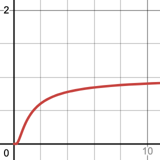
is a prototypical example of a test function. It was used in the proof of the non-existence of the Dirac delta function above. The exponential function is, by one of its definitions, a fixed point of differentiation (i.e., it equals its derivative), and hence is infinitely differentiable. Its graph looks like

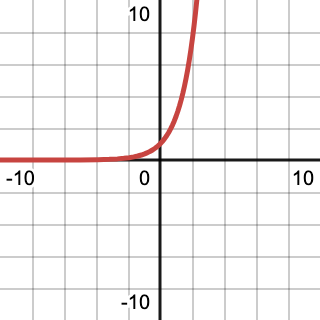
The graph of \(e^{-\frac{1}{x}}\) is "rotated" so that the asymptote occurs horizontally.

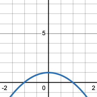
The function \(1 - x^2\) is an "arc" that crosses \(y=0\) at \(x=1\) and \(x=-1\).

By composing \(1-x^2\) with \(e^{-\frac{1}{x}}\), we obtain \(e^{\frac{1}{x^2 - 1}}\).

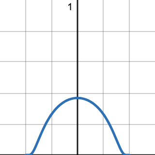
Together, when restricted to values with \(\lvert x \rvert < 1\), this produces a function with all the desired properties: it is smooth (infinitely differentiable) and it vanishes outside a compact interval \([-1, 1]\).

Due to the shape of such functions, they are often called bump functions. Although such functions enjoy special properties (and producing explicit examples can be tricky), there is an abundance of such functions, since, once we establish the existence of some stock of test functions, we can produce additional test functions via the following operations:

• Linear combinations: \(c_1 \cdot \varphi_1 + \dots + c_n \cdot \varphi_n\),
• Scaling: \(\varphi(c \cdot x)\),
• Translation: \(\varphi(x - a)\),
• Partial differentiation.

Definition (Locally Integrable Function). A function \(f : \mathbb{R}^n \rightarrow \mathbb{C}\) is locally integrable if, for every compact set \(K \subset\mathbb{R}^n\)

\[\int_K \lvert f(\bar{x}) \rvert ~d\bar{x} \lt \infty.\]

Theorem. For any two locally integrable functions \(f, g : \mathbb{R}^n \rightarrow \mathbb{C}\), \(f = g\) almost everywhere if and only if for every test function \(\varphi : \mathbb{R}^n \rightarrow \mathbb{C}\),

\[\int_K f(\bar{x})\cdot \varphi(\bar{x})~d\bar{x} = \int_K g(\bar{x})\cdot \varphi(\bar{x})~d\bar{x}.\]

Proof. Laurent Schwartz, the pioneer of the theory of distributions, provides a proof in his book Mathematics for the Physical Sciences.

By "almost everywhere" we mean that the set \(\{\bar{x} \in \mathbb{R}^n : f(\bar{x}) \ne g(\bar{x})\}\) has Lebesgue measure \(0\).

Thus, for any locally integrable function \(f : \mathbb{R}^n \rightarrow. \mathbb{C}\), we can define a canonical operation \(D_f : \mathcal{D}(\mathbb{R}^n) \rightarrow \mathbb{C}\) as follows:

\[D_f(\varphi) = \int_{\mathbb{R}^n} f(\bar{x})\cdot \varphi(\bar{x})~d\bar{x}.\]

Note that, although the domain of integration is now the entirety of \(\mathbb{R}^n\), since each \(\varphi\) vanishes outside some compact set, this is effectively an integral over this compact set.

Thus, functions \(f\) can be re-interpreted according to their canonical actions \(D_f\) upon test functions.

Thus, two functions are the same (modulo a set of measure \(0\)) if and only if their respective operations \(D_f\) and \(D_g\) coincide.

This provides an avenue toward generalization: the operations \(D_f\) are maps with signature \(\mathcal{D}(\mathbb{R}^n) \rightarrow \mathbb{C}\). Instead of restricting ourselves to the particular maps \(D_f\), we can instead consider any such map satisfying appropriate conditions. Thus, a "generalized function" will be a map from test functions into complex numbers (where, of course, they can be maps into real numbers as well since \(\mathbb{R} \subset \mathbb{C}\)). The maps \(D_f\) are both linear and continuous (in an appropriate sense), so we make the following definition.

Definition (Distribution). A distribution is a continuous linear map \(D : \mathcal{D}(\mathbb{R}^n) \rightarrow \mathbb{C}\).

By linear we mean, as usual, that

• \(D(\varphi + \psi) = D(\varphi) + D(\psi)\) and
• \(D(a \cdot \varphi) = a \cdot D(\varphi)\)

for all test functions \(\varphi, \psi \in \mathcal{D}(\mathbb{R}^n)\) and real numbers \(\mathbb{R}\).

Often the notation \(\langle D, \varphi\rangle = D(\varphi)\) is used to denote the action of a distribution \(D\) on a test function \(\varphi\).

By continuous, we mean, as usual, that \(D(\varphi_n) \downarrow D(\varphi)\) whenever \(\varphi_n \downarrow \varphi\) for every sequence \((\varphi_n)_{n \in \mathbb{N}}\) (i.e., continuous functions are homomorphisms that preserve convergence).

Note that it is possible to define continuity as follows: \(D(\varphi_n) \downarrow 0\) whenever \(\varphi_n \downarrow 0\), since \(\varphi_n \downarrow \varphi\) if and only if \(\varphi_n - \varphi \downarrow 0\). To see this, suppose that \(D\) is continuous according to this alternative definition and suppose that \(\varphi_n \downarrow \varphi\). Then \(\varphi_n - \varphi \downarrow 0\), and thus, by the alternative definition of continuity, \(D(\varphi_n - \varphi) \downarrow 0\). By the linearity of \(D\), \(D(\varphi_n) - D(\varphi) \downarrow 0\), and thus, \(D(\varphi_n) \downarrow D(\varphi)\).

However, we must explain what is meant by convergence in this context.

Definition (Convergence in \(\mathcal{D}(\mathbb{R}^n)\)). A sequence of test functions \((\varphi_n)_{n \in \mathbb{N}}\) converges to a test function \(\varphi \in \mathcal{D}(\mathbb{R}^n)\) if the following conditions are satisfied:

• There exists a compact set \(K\) such that every \(\varphi_n\) vanishes (is \(0\)) outside \(K\), and
• The sequence \((\varphi_n)_{n \in \mathbb{N}}\) converges uniformly to \(\varphi\), i.e., for every \(\varepsilon > 0\), there exists an \(N \in \mathbb{N}\) such that, for all \(n > N\) and all \(\bar{x} \in K\), \(\lvert \varphi_n(\bar{x}) - \varphi(\bar{x}) \rvert \lt \varepsilon\), and
• For each multi-index \(k\), \(D^k\varphi_n\) converges uniformly to \(D^k\varphi\).

By a multi-index we mean a tuple of integers \((k_1,\dots,k_n)\) such that \(k_1,\dots,k_n \in [1, \infty)\) and the notation \(D^k\) denotes the following partial derivative operation (with respective to coordinate functions \(x_1,\dots,x_n\)):

\[\frac{\partial^{k_1 + \dots + k_n}}{\partial x_1^{k_1} \dots \partial x_n^{k_n}}.\]

This notation simply represents all possible partial derivatives of all orders.

Thus, every function \(f : \mathbb{R}^n \rightarrow \mathbb{C}\) yields a distribution \(D_f\); we call such distributions regular distributions.

We can now demonstrate that the regular distributions \(D_f\) are indeed continuous. Suppose that \(\varphi_n \downarrow 0\) and that all \(\varphi_n\) vanish outside some compact set \(K\).

\begin{align*}\lvert \langle D_f, \varphi_n \rangle \rvert &= \left\lvert\int_{\mathbb{R}^n}f(\bar{x})\varphi_n(\bar{x})~d\bar{x}\right\rvert \\&= \left\lvert\int_K f(\bar{x})\varphi_n(\bar{x})~d\bar{x} \right\rvert\\&\le \int_{K}\lvert f(\bar{x})\rvert \lvert \varphi_n(\bar{x})\rvert~d\bar{x} \\&\le \int_K \lvert f(\bar{x})\rvert \lVert \varphi_n \rVert_{\infty}~d\bar{x} \\&= \lVert \varphi_n \rVert_{\infty} \cdot \int_K \lvert f(\bar{x})\rvert ~d\bar{x}.\end{align*}

Here \(\lVert \cdot \rVert_{\infty}\) denotes the supremum norm. Since \(\varphi_n \downarrow 0\), it follows that \(\lVert \varphi_n \rVert \downarrow 0\), and thus, the above expression likewise converges to \(0\). The value of \(\langle D_f, \varphi_n \rangle\) is just \(0\), so \(\langle D_f, \varphi_n \rangle \downarrow \langle D_f,0\rangle\), as required.

However, we can also define distributions which are not regular, and indeed this is one of the primary purposes of distributions. The Dirac delta is a prime example. We may define the Dirac delta distribution as follows.

Definition (Dirac Delta Distribution). The Dirac delta distribution is the distribution \(\delta_{\bar{a}}\) defined for some \(\bar{a} \in \mathbb{R}^n\) and every test function \(\varphi\) as

\[\delta_{\bar{a}}(\varphi) = \varphi(\bar{a}).\]

This is indeed linear, since operations on test functions are defined point-wise, i.e.,

• \(\delta_{\bar{a}}(\varphi + \psi) = (\varphi + \psi)(\bar{a}) = \varphi(\bar{a}) + \psi(\bar{a})\) and
• \(\delta_{\bar{a}}(c \cdot \varphi) = (c \cdot \varphi)(\bar{a}) = c \cdot \varphi(\bar{a})\).

This is also continuous, since it is defined point-wise; uniform convergence means that, for every element \(\bar{x} \in \mathbb{R}^n\), the point-wise sequence \((\varphi_n(\bar{x}))_{n \in \mathbb{N}}\) converges to \(\varphi(\bar{x})\). Thus, if \(\varphi_n \downarrow \varphi\), then \(\varphi_n(\bar{x}) \downarrow \varphi(\bar{x})\), which, by definition, means that \(\delta_{\bar{a}}(\varphi_n) \downarrow \delta_{\bar{a}}(\varphi)\).

Distributional Derivatives

Distributions allow us to define a generalization of differentiation (i.e., to define an appropriate notion of the derivative of functions which are not classically differentiable).

Note that, for any locally integrable function \(f : \mathbb{R} \rightarrow \mathbb{R}\) and any test function \(\varphi\) which vanishes outside \([a,b]\) by applying integration by parts, it follows that

\begin{align*}\langle D_{f'}, \varphi \rangle &= \int_{\mathbb{R}^n}f'(\bar{x})\varphi(\bar{x})~d\bar{x} \\&= \int_a^bf'(\bar{x})\varphi(\bar{x})~d\bar{x} \\&= \left[ f(\bar{x})\varphi(\bar{x})\right]_a^b - \int_a^bf(\bar{x})\varphi'(\bar{x})~d\bar{x} \\&= - \int_a^bf(\bar{x})\varphi'(\bar{x})~d\bar{x} \\&= -\langle D_f, \varphi'\rangle.\end{align*}

Here, we used the fact that \(\varphi(a) = \varphi(b) = 0\) since \(\varphi\) is continuous and vanishes outside \([a,b]\).

This suggests the following definition.

Definition (Distributional Derivative). The distributional derivative \(D'\) of a distribution \(D \in \mathcal{D}'(\mathbb{R})\) is defined for every \(\varphi \in \mathcal{D}(\mathbb{R})\) by the action

\[\langle D', \varphi \rangle = -\langle D, \varphi' \rangle.\]

As we previously demonstrated, \(\langle (D_f)', \varphi \rangle = \langle D_{f'}, \varphi \rangle\), and thus \((D_f)' = D_{f'}\), so the distributional derivative is a conservative extension of the classical derivative in precisely this sense.

Note that the definition is well-defined: if \(\varphi \in \mathcal{D}(\mathbb{R})\), then, since \(\mathcal{D}(\mathbb{R})\) is closed under partial differentiation (and the classical derivative is a special case of partial differentiation), it follows that \(\varphi' \in \mathcal{D}(\mathbb{R})\).

The distributional derivative is indeed linear, since

\begin{align*}\langle D', \varphi + \psi \rangle &= -\langle D, (\varphi + \psi)' \rangle \\&= -\langle D, \varphi' + \psi'\rangle \\&= -(\langle D, \varphi' \rangle + \langle D, \psi') \\&= -\langle D, \varphi' \rangle - \langle D, \psi' \rangle \\&= \langle D', \varphi \rangle + \langle D', \psi \rangle.\end{align*}

and

\begin{align*}\langle D', a \cdot \varphi \rangle &= - \langle D, (a \cdot \varphi)' \rangle \\&= -\langle D, a \cdot \varphi' \rangle \\&= -a \cdot \langle D, \varphi' \rangle \\&= a \cdot \langle D', \varphi \rangle.\end{align*}

The distributional derivative is indeed continuous as well, since, if \(\varphi_n \downarrow 0\), then, by definition of convergence in \(\mathcal{D}(\mathbb{R})\), \(\varphi_n' \downarrow 0\) (since the classical derivative is just a one-dimensional partial derivative), and thus \(\langle D, \varphi_n' \rangle \downarrow \langle D, 0 \rangle\) (since \(D\) is a distribution and hence continuous). It then follows that \(-\langle D, \varphi_n' \rangle \downarrow -\langle D, 0 \rangle\) and thus \(\langle D', \varphi_n \rangle \downarrow \langle D', 0 \rangle\).

Example. The distributional derivative \(\delta'\) of the Dirac delta distribution \(\delta\) is called the dipole, and is defined as follows:

\[\langle \delta', \varphi \rangle = -\langle \delta, \varphi' \rangle = -\varphi'(0).\]

Example. The Heaviside step function \(H : \mathbb{R}/\{0\} \rightarrow \mathbb{R}\) is defined as follows:

\[H(x) = \begin{cases}1 & \text{if \(x > 0\)} \\ 0 & \text{if \(x < 0\)}\end{cases}\]

Note that the Heaviside step function is locally integrable and hence there is a corresponding regular distribution

\[\langle D_H, \varphi \rangle = \int_{\mathbb{R}}H(x)\varphi(x)~dx.\]

We compute its distributional derivative as follows:

\begin{align*}\langle (D_H)', \varphi \rangle &= -\langle D_H, \varphi'\rangle \\&= -\int_{\mathbb{R}}H(x)\varphi'(x)~dx \\&= \int_0^{\infty}\varphi'(x)~dx \\&= \lim_{b \to \infty}\left(-\int_0^b \varphi'(x)~dx\right) \\&= \lim_{b \to \infty}(-(\varphi(b) - \varphi(0))) \\&= -\lim_{b \to \infty}(\varphi(b) - \varphi(0)) \\&= -(\lim_{b \to \infty}\varphi(b) - \lim_{b \to \infty}\varphi(0)) \\&= -(0 - \varphi(0)) \\&= \varphi(0) \\&= \langle \delta, \varphi \rangle.\end{align*}

This shows that \((D_H)' = \delta\), i.e., the distributional derivative of the Heaviside distribution is the Dirac delta distribution.

We can extend the definition of distributional derivatives to define distributional partial derivatives.

Definition (Distributional partial derivatives). The \(i\)-th distributional partial derivative \((\partial D/\partial x^i)\) of a distribution \(D \in \mathcal{D}'(\mathbb{R}^n)\) is defined for each \(\varphi \in \mathcal{D}(\mathbb{R}^n)\) as

\[\left\langle \frac{\partial D}{\partial x^i}, \varphi \right\rangle = -\left\langle D, \frac{\partial \varphi}{\partial x^i} \right\rangle.\]

Note that this essentially the same as the previous definition (since the classical derivative is a special case of the partial derivative).

The distributional partial derivative enjoys several properties in common with the classical partial derivative. For instance,

\begin{align*}\left\langle \frac{\partial^2 D}{\partial x^i \partial x^j}, \varphi \right\rangle &= \left\langle \frac{\partial}{\partial x^i}\left(\frac{\partial D}{\partial x^j}\right), \varphi \right \rangle \\&= -\left\langle \frac{\partial D}{\partial x^j}, \frac{\partial \varphi}{\partial x^i} \right\rangle \\&= -\left(-\left\langle D, \frac{\partial^2 \varphi}{\partial x^j \partial x^i}\right\rangle\right) \\&= \left\langle D, \frac{\partial^2 \varphi}{\partial x^j \partial x^i}\right\rangle \\&= \left\langle D, \frac{\partial^2 \varphi}{\partial x^i \partial x^j}\right\rangle.\end{align*}

From this last equation, we infer that

\[\frac{\partial^2 D}{\partial x^i \partial x^j} = \frac{\partial^2 D}{\partial x^j \partial x^i}.\]

Since \(\mathcal{D}'(\mathbb{R}^n)\) is a vector space, we can define linear map \((\partial/\partial x^i)\) for any \(D \in \mathcal{D}'(\mathbb{R}^n)\) as follows:

\[\frac{\partial}{\partial x^i}(D) = \frac{\partial D}{\partial x^i}.\]

Note that

\begin{align*}\left\langle\frac{\partial}{\partial x^i}(D_1 + D_2),\varphi \right\rangle &= \left \langle\frac{\partial (D_1 + D_2)}{\partial x^i}, \varphi \right \rangle \\&= -\left\langle D_1 + D_2, \frac{\partial \varphi}{\partial x^i}\right\rangle \\&= -\left( \left\langle D_1, \frac{\partial \varphi}{\partial x^i}\right\rangle + \left\langle D_2, \frac{\partial \varphi}{\partial x^i} \right\rangle\right) \\&= -\left\langle D_1, \frac{\partial \varphi}{\partial x^i}\right\rangle - \left\langle D_2, \frac{\partial \varphi}{\partial x^i} \right\rangle \\&= \left\langle \frac{\partial D_1}{\partial x^i}, \varphi\right\rangle + \left\langle \frac{\partial D_2}{\partial x^i},\varphi \right\rangle \\&= \left\langle \frac{\partial}{\partial x^i}(D_1), \varphi\right\rangle + \left\langle \frac{\partial}{\partial x^i}(D_2),\varphi \right\rangle.\end{align*}

Also note that

\begin{align*}\left\langle \frac{\partial}{\partial x^i}(c \cdot D), \varphi \right\rangle &= \left\langle \frac{\partial (c \cdot D)}{\partial x^i} \right\rangle \\&= -\left\langle c \cdot D, \frac{\partial \varphi}{\partial x^i}\right\rangle \\&= -c \cdot \left\langle D, \frac{\partial \varphi}{\partial x^i}\right\rangle \\&= c \cdot \left\langle \frac{\partial D}{\partial x^i}, \varphi \right\rangle \\&= c \cdot \left\langle \frac{\partial}{\partial x^i}(D), \varphi \right\rangle.\end{align*}

Thus, the map \((\partial / \partial x^i)\) is indeed a linear map.

The set of all distributional partial derivatives forms a vector space also under point-wise addition and scalar multiplication.

Weak PDE Solutions

We will now give an example indicating how distributions can provide weak solutions to partial differential equations. By a weak solution, we mean a solution to the corresponding distributional equation which is merely locally integrable (as opposed to a classical solution which must be classically differentiable).

Example.

As an example, we will indicate a weak solution to the wave equation

\[\frac{\partial^2 u}{\partial t^2} - \frac{\partial^2 u}{\partial x^2} = 0.\]

First, we will prove a technical lemma. We will first consider the equation

\[\frac{\partial u}{\partial t} - c \cdot \frac{\partial u}{\partial x} = 0\]

with the initial condition \(u(x, 0) = f(x)\). When \(f \in C^1\), a classical solution is given by

\[u(x,t) = f(x + c \cdot t)\]

since

\[u(x, 0) = f(x + 0 \cdot t) = f(x)\]

and, for all \(x,t \in \mathbb{R}\),

\begin{align*}\left(\frac{\partial u}{\partial t} - c \cdot \frac{\partial u}{\partial x}\right)(x,t) &= f'(x + c \cdot t) \cdot c - c \cdot f'(x + c \cdot t) \\&= 0.\end{align*}

However, even when \(f\) is merely locally integrable, the regular distribution \(D_u\) is a distributional solution to the same equation. For any \(\varphi \in \mathcal{D}(\mathbb{R}^2)\),

\begin{align*}\left\langle \frac{\partial D_u}{\partial t} - c \cdot \frac{\partial D_u}{\partial x}, \varphi \right\rangle &= \left\langle \left(\frac{\partial}{\partial t} - c \cdot \frac{\partial}{\partial x}\right) D_u, \varphi \right\rangle \\&= -\left\langle D_u, \frac{\partial \varphi}{\partial t} - c \cdot \frac{\partial \varphi}{\partial x}\right\rangle \\&= \left\langle D_u, c \cdot \frac{\partial \varphi}{\partial x} - \frac{\partial \varphi}{\partial t}\right\rangle \\&= \int_{\mathbb{R}^2}f(x + c \cdot t) \cdot \left(c \cdot \frac{\partial \varphi}{\partial x} - \frac{\partial \varphi}{\partial t} \right)(x,t)~dx~dt\end{align*}

We will write this ultimate expression in terms of a function \(G : \mathbb{R}^2 \rightarrow \mathbb{R}\) as

\[\int_{\mathbb{R}^2}f(x + c \cdot t) \cdot \left( c \cdot \frac{\partial \varphi}{\partial x} - \frac{\partial \varphi}{\partial t}\right)(x,t)~dx~dt = \int_{\mathbb{R}^2}G(x, t)~dx~dt\]

where

\[G(x,t) = f(x + c \cdot t) \cdot \left(c \cdot \frac{\partial \varphi}{\partial x} - \frac{\partial \varphi}{\partial t} \right)(x,t).\]

The expression

\[\left( c \cdot \frac{\partial \varphi}{\partial x} - \frac{\partial \varphi}{\partial t}\right)(x,t)\]

is very similar to the expression for the chain rule for partial derivatives, namely, for a function \(F : \mathbb{R}^2 \rightarrow \mathbb{R}^2\),

\[\frac{\partial (\varphi \circ F)}{\partial y_2} = \frac{\partial F^1}{\partial y_2}(y_1, y_2) \cdot \frac{\partial \varphi}{\partial x}(F(y_1, y_2)) + \frac{\partial F^2}{\partial y_2}(y_1, y_2) \cdot \frac{\partial \varphi}{\partial t}(F(y_1, y_2)).\]

If we choose the function

\[F(y_1, y_2) = (y_1 - c \cdot y_2, y_2),\]

then we compute

\[\frac{\partial (\varphi \circ F)}{\partial y_2} = -c \cdot \frac{\partial \varphi}{\partial x}(y_1 - c \cdot y_2, y_2) + 1 \cdot \frac{\partial \varphi}{\partial t}(y_1 + c \cdot y_2, y_2).\]

Extracting a term of \(-1\), we then obtain

\[-\frac{\partial (\varphi \circ F)}{\partial y_2} = c \cdot \frac{\partial \varphi}{\partial x}(y_1 - c \cdot y_2, y_2) - \frac{\partial \varphi}{\partial t}(y_1 + c \cdot y_2, y_2).\]

Thus, if we perform a change of variables (i.e., a pullback), we get, using the standard formula,

\[\int_{\mathbb{R}^2}G(x, t)~dx~dt = \int_{\mathbb{R}^2}(G \circ F)(y_1, y_2) \cdot \lvert \mathrm{det}(JF) \rvert~dy_1~dy_2,\]

where \(JF\) denotes the Jacobian matrix and is defined as follows:

\[JF = \begin{bmatrix}\frac{\partial F^1}{\partial y_1} & \frac{\partial F^1}{\partial y_2} \\ \frac{\partial F^2}{\partial y_1} & \frac{\partial F^2}{\partial y_1}\end{bmatrix} = \begin{bmatrix}1 & -c \\ 0 & 1\end{bmatrix}.\]

Thus, \(\mathrm{det}(JF) = 1\).

With the expression converted to a single partial derivative, we can apply the fundamental theorem of calculus. We then continue to compute:

\begin{align*}\int_{\mathbb{R}^2}G(x, t)~dx~dt &= \int_{\mathbb{R}^2}(G \circ F)(y_1, y_2) \cdot \lvert \mathrm{det}(JF) \rvert~dy_1~dy_2 \\&= \int_{\mathbb{R}^2}f((y_1 - c \cdot y_2) + c \cdot y_2) \cdot \left(c \cdot \frac{\partial \varphi}{\partial x}(y_1 + c \cdot y_2, y_2) - \frac{\partial \varphi}{\partial t}(y_1 + c \cdot y_2, y_2)\right) \cdot \lvert 1 \rvert ~dy_1~dy_2 \\&= \int_{\mathbb{R}^2}-f(y_1) \cdot \left(-c \cdot \frac{\partial \varphi}{\partial x}(y_1 + c \cdot y_2, y_2) + \frac{\partial \varphi}{\partial t}(y_1 + c \cdot y_2, y_2)\right) ~dy_1~dy_2 \\&= \int_{\mathbb{R}^2}-f(y_1) \cdot \frac{\partial (\varphi \circ F)}{\partial y_2}(y_1, y_2) ~dy_1~dy_2 \\&= -\int_{-\infty}^{\infty}\int_{-\infty}^{\infty}f(y_1) \cdot \frac{\partial (\varphi \circ F)}{\partial y_2}(y_1, y_2)~dy_1~dy_2 \\&= -\int_{-\infty}^{\infty}f(y_1) \cdot \left(\int_{-\infty}^{\infty} \frac{\partial (\varphi \circ F)}{\partial y_2}(y_1, y_2) ~dy_2\right)~dy_1 \\&= -\int_{-\infty}^{\infty}f(y_1) \cdot \left(\lim_{y_2 \to \infty}(\varphi \circ F)(y_1, y_2) - \lim_{y_2 \to -\infty} (\varphi \circ F)(y_1, y_2)\right)~dy_1 \\&= -\int_{-\infty}^{\infty}f(y_1) \cdot \left(\lim_{y_2 \to \infty}\varphi(y_1 + c \cdot y_2, y_2) - \lim_{y_2 \to -\infty} \varphi(y_1 + c \cdot y_2, y_2)\right)~dy_1 \\&= -\int_{-\infty}^{\infty}f(y_1) \cdot \left(0 - 0\right)~dy_1 \\&= -\int_{-\infty}^{\infty}f(y_1) \cdot 0 ~dy_1 \\&= 0.\end{align*}

Note that the limits are \(0\) because \(\varphi\) has compact support, and thus is \(0\) outside this support.

Thus, we have demonstrated that, for all \(\varphi \in \mathcal{D}(\mathbb{R}^2)\),

\[\left\langle \frac{\partial D_u}{\partial t} - c \cdot \frac{\partial D_u}{\partial x}, \varphi \right\rangle = 0,\]

and hence

\[\frac{\partial D_u}{\partial t} - c \cdot \frac{\partial D_u}{\partial x} = 0\]

and \(D_u\) is a distributional solution to the PDE.

Now, returning to the wave equation, first note the following:

\begin{align*}\left(\frac{\partial}{\partial t} - \frac{\partial}{\partial x}\right)\left(\left(\frac{\partial}{\partial t} + \frac{\partial}{\partial x}\right)(D)\right) &= \left(\frac{\partial}{\partial t} - \frac{\partial}{\partial x}\right)\left(\frac{\partial D}{\partial t} + \frac{\partial D}{\partial x}\right) \\&= \left(\frac{\partial}{\partial t}\left(\frac{\partial D}{\partial t} + \frac{\partial D}{\partial x}\right) - \frac{\partial}{\partial x}\left(\frac{\partial D}{\partial t} + \frac{\partial D}{\partial x}\right)\right) \\&= \left(\frac{\partial}{\partial t}\left(\frac{\partial D}{\partial t}\right) + \frac{\partial}{\partial t}\left( \frac{\partial D}{\partial x}\right) - \frac{\partial}{\partial x}\left(\frac{\partial D}{\partial t}\right) - \frac{\partial}{\partial x}\left(\frac{\partial D}{\partial x}\right)\right) \\&= \left(\frac{\partial}{\partial t}\left(\frac{\partial D}{\partial t}\right) - \frac{\partial}{\partial x}\left(\frac{\partial D}{\partial x}\right)\right) \\&= \frac{\partial^2 D}{\partial t^2} - \frac{\partial^2 D}{\partial x^2}.\end{align*}

A similar calculation shows that

\[\left(\frac{\partial}{\partial t} - \frac{\partial}{\partial x}\right) \left(\left(\frac{\partial}{\partial t} + \frac{\partial}{\partial x}\right)(D)\right) = \frac{\partial^2 D}{\partial t^2} - \frac{\partial^2 D}{\partial x^2}.\]

Now, for any locally integrable function \(f\), the regular distribution \(D_{u^+}\) corresponding to the function \(u^+(x,t) = f(x + t)\) is a solution (with \(c=1\)) to

\[\frac{\partial D_{u^+}}{\partial t} - \frac{\partial D_{u^+}}{\partial x} = 0
.\]

Likewise, the regular distribution \(D_{u^-}\) corresponding to the function \(u^-(x,t) = f(x - t)\) is a solution (with \(c = -1\)) to

\[\frac{\partial D_{u^+}}{\partial t} + \frac{\partial D_{u^+}}{\partial x} = 0
.\]

We will show that \(D_u\), where

\[u(x,t) = \frac{u^+ + u^-}{2} = \frac{f(x + t) + f(x - t)}{2}\]

is a distributional solution to the equation

\[\frac{\partial^2 D_u}{\partial t^2} - \frac{\partial^2 D_u}{\partial x^2} = 0.\]

Note that, for any locally integrable functions \(f,g\),

\begin{align*}\langle D_{f+g}, \varphi \rangle &= \int_{\mathbb{R}^n}(f+g)(x) \cdot \varphi(x)~dx \\&= \int_{\mathbb{R}^n}(f(x)+g(x)) \cdot \varphi(x)~dx \\&= \int_{\mathbb{R}^n}(f(x) \cdot \varphi(x))~dx + \int_{\mathbb{R}^n}(g(x) \cdot \varphi(x))~dx \\&= \langle D_f, \varphi \rangle + \langle D_g, \varphi \rangle\end{align*}

and thus \(D_{f+g} = D_f + D_g\). Likewise, \(D_{a \cdot f} = a \cdot D_f\), so \(D_{(-)}\) is a linear operation.

We calculate the following:

\begin{align*}\left\langle \frac{\partial^2 D_u}{\partial t^2} - \frac{\partial^2 D_u}{\partial x^2}, \varphi \right\rangle &= \left\langle \left(\frac{\partial^2}{\partial t^2} - \frac{\partial^2}{\partial x^2}\right)D_u,\varphi \right\rangle \\&= \left\langle \left(\frac{\partial^2}{\partial t^2} - \frac{\partial^2}{\partial x^2}\right)D_{\frac{1}{2} \cdot (u^+ + u^-)},\varphi \right\rangle \\&= \left\langle \left(\frac{\partial^2}{\partial t^2} - \frac{\partial^2}{\partial x^2}\right)\left(\frac{1}{2} \cdot D_{(u^+ + u^-)}\right),\varphi \right\rangle \\&= \left\langle \frac{1}{2} \cdot \left(\frac{\partial^2}{\partial t^2} - \frac{\partial^2}{\partial x^2}\right)D_{(u^+ + u^-)},\varphi \right\rangle \\&= \frac{1}{2} \cdot \left\langle \left(\frac{\partial^2}{\partial t^2} - \frac{\partial^2}{\partial x^2}\right)D_{(u^+ + u^-)},\varphi \right\rangle \\&= \frac{1}{2} \cdot \left\langle \left(\frac{\partial^2}{\partial t^2} - \frac{\partial^2}{\partial x^2}\right)\left(D_{u^+} + D_{u^-}\right),\varphi \right\rangle \\&= \frac{1}{2} \cdot \left\langle \left(\frac{\partial^2}{\partial t^2} - \frac{\partial^2}{\partial x^2}\right)D_{u^+} + \left(\frac{\partial^2}{\partial t^2} - \frac{\partial^2}{\partial x^2}\right)D_{u^-},\varphi \right\rangle \\&= \frac{1}{2} \cdot \left\langle \left(\frac{\partial^2}{\partial t^2} - \frac{\partial^2}{\partial x^2}\right)D_{u^+}, \varphi \right\rangle \\&+ \frac{1}{2} \cdot \left\langle \left(\frac{\partial^2}{\partial t^2} - \frac{\partial^2}{\partial x^2}\right)D_{u^-},\varphi \right\rangle \\&= \frac{1}{2} \cdot \left\langle \left(\frac{\partial}{\partial t} + \frac{\partial}{\partial x}\right)\left(\frac{\partial}{\partial t} - \frac{\partial}{\partial x}\right)D_{u^+}, \varphi \right\rangle \\&+ \frac{1}{2} \cdot \left\langle \left(\frac{\partial}{\partial t} - \frac{\partial}{\partial x}\right)\left(\frac{\partial}{\partial t} + \frac{\partial}{\partial x}\right)D_{u^-},\varphi \right\rangle \\&= -\frac{1}{2} \cdot \left\langle \left(\frac{\partial}{\partial t} - \frac{\partial}{\partial x}\right)D_{u^+}, \frac{\partial \varphi}{\partial t} + \frac{\partial \varphi}{\partial x} \right\rangle \\&- \frac{1}{2} \cdot \left\langle \left(\frac{\partial}{\partial t} + \frac{\partial}{\partial x}\right)D_{u^-}, \frac{\partial \varphi}{\partial t} - \frac{\partial \varphi}{\partial x} \right\rangle \\&= -\frac{1}{2} \cdot \left\langle 0, \frac{\partial \varphi}{\partial t} + \frac{\partial \varphi}{\partial x} \right\rangle \\&- \frac{1}{2} \cdot \left\langle 0, \frac{\partial \varphi}{\partial t} - \frac{\partial \varphi}{\partial x} \right\rangle \\&= -\frac{1}{2} \cdot 0 - \frac{1}{2} \cdot 0 \\&= 0.\end{align*}

Thus, \(D_u\) is indeed a distributional solution to the PDE.

Modular Structure

The multiplication of a smooth function \(f \in C^{\infty}(\mathbb{R}^n)\) with a distribution \(D \in \mathcal{D}'(\mathbb{R}^n)\) is defined as follows for all \(\varphi \in \mathcal{D}(\mathbb{R}^n)\):

\[\langle f \cdot D, \varphi \rangle = \langle D, f \cdot \varphi \rangle.\]

First, note that for \(\varphi \in \mathcal{D}(\mathbb{R}^n)\) and \(f \in C^{\infty}(\mathbb{R}^n)\), the product \(f \cdot \varphi\) is smooth since each of \(f\) \and \(\varphi\) is smooth, and, since \(\varphi\) has compact support, so does \(f \cdot \varphi\).

Next, note that

\begin{align*}\langle f \cdot D, \varphi + \psi \rangle &= \langle D, f \cdot (\varphi + \psi) \rangle \\&= \langle D, f \cdot \varphi + f \cdot \psi \rangle \\&= \langle D, f \cdot \varphi \rangle + \langle D, f \cdot \psi \rangle\end{align*}

and

\begin{align*}\langle f \cdot D, a \cdot \varphi \rangle &= \langle D, f \cdot (a \cdot \varphi) \rangle \\&= a \cdot \langle D, f \cdot \varphi \rangle \end{align*}

and thus the map \(f \cdot D\) is linear, as required.

The map \(f \cdot D\) is also continuous. There is a multivariable version of the Leibniz rule which states that

\[D^n(fg) = \sum_K \binom{\lvert n \rvert}{\lvert k \rvert}(D^k f)(D^{n - k}g)\]

where

\[K = \{(k_1, \dots, k_d) : k_i \le n_i, i \in \{1, \dots, d\}\}\]

is the set of all relevant multi-indices,

\[\lvert n \rvert = \sum_i n_i,\]

and

\[(n - k) = (n_i - k_i, \dots, n_d - k_d)\]

and

\[D^n = \frac{\partial^{\lvert n \rvert}}{\partial x_1^{n_1} \dots \partial x_d^{n_d}}\]

and

\[\binom{n}{k} = \frac{n!}{k!(n - k)!}.\]

Using the Leibniz rule, if \(\varphi_n \downarrow 0\), then \(f \cdot \varphi_n \downarrow 0\) also. Thus, the map \(f \cdot D\) is continuous, as required.

Equipped with this multiplication operation, the space of all distributions \(\mathcal{D}'(\mathbb{R}^n)\) is a module over the ring \(C^{\infty}(\mathbb{R}^n)\). In particular, this means that

• \(f \cdot (D_1 + D_2) = f \cdot D_1 + f \cdot D_2\),
• \((f_1 + f_2) \cdot D = f_1 \cdot D + f_2 \cdot D\),
• \((f_1f_2) \cdot D = f_1 \cdot (f_2 \cdot D)\),
• \(1 \cdot D = D\).

Fourier Transforms

The classical Fourier theory can be extended to so-called tempered distributions. Here, we will briefly outline the main ideas.

Suppose that we have some function \(f\) whose Fourier transform and regular distribution \(D_f\) is well-defined (e.g. an absolutely integrable function). We will write \(\hat{f}\) for the Fourier transform of \(f\), which is defined as follows:

\[\hat{f}(\xi) = \int_{-\infty}^{\infty}f(x) \cdot e^{-2\pi i \xi x}~dx.\]

For regular distributions we will make the definition

\[\left \langle \widehat{D_f}, \varphi \right \rangle = \left \langle D_{\hat{f}}, \varphi \right \rangle.\]

Then, assuming that \(\hat{\varphi}\) has compact support, we tentatively compute the following:

\begin{align*}\left \langle \widehat{D_f}, \varphi \right \rangle &= \left \langle D_{\hat{f}}, \varphi \right \rangle \\&= \int_{-\infty}^{\infty} \varphi(x) \cdot \hat{f}(x)~dx \\&= \int_{-\infty}^{\infty} \varphi(x) \cdot \left(\int_{-\infty}^{\infty}f(\xi) \cdot e^{-2\pi i \xi x}~d\xi\right)~dx \\&= \int_{-\infty}^{\infty} f(\xi) \cdot \left(\int_{-\infty}^{\infty}\varphi(x) \cdot e^{-2\pi i \xi x}~dx\right)~d\xi \\&= \left \langle T_f, \hat{\varphi} \right \rangle.\end{align*}

However, the space of test functions \(\mathcal{D}(\mathbb{R})\) is not closed under the Fourier transform. If it were, however, we could define the Fourier transform of an arbitrary distribution \(D\) as

\[\left \langle \hat{D}, \varphi \right \rangle = \left \langle D, \hat{\varphi} \right \rangle.\]

Note the similarity to the definition of the derivative.

The strategy will be to enlarge the class of test functions such that this new class of test functions is closed under the Fourier transform. This new space of test functions is often called the Schwartz space in honor of Laurent Schwartz (the pioneer of distribution theory). Here, we'll just indicate the definition for \(\mathbb{R}\), but it can be extended to \(\mathbb{R}^n\).

Definition (Schwartz Space). The Schwartz space of test functions \(\mathcal{S}(\mathbb{R})\) is the set of all functions \(\varphi : \mathbb{R} \rightarrow \mathbb{C}\) satisfying the following conditions:

1. \(\varphi\) is smooth,
2. for all \(\ell, m \in \mathbb{N}\), \(\sup_{x \in \mathbb{R}}\lvert x^{\ell} \varphi^{(m)}(x) \rvert \lt +\infty\).

Note that \(\mathcal{S}(\mathbb{R})\) is a real vector space using point-wise addition and scalar multiplication.

For every test function \(\varphi \in \mathcal{D}(\mathbb{R})\), since \(\varphi\) has compact support, it follows that \(\sup_{x \in \mathbb{R}}\lvert x^{\ell} \varphi^{(m)} \rvert \lt +\infty\), and hence \(\varphi \in \mathcal{S}(\mathbb{R})\), so \(\mathcal{D}(\mathbb{R}) \subset \mathcal{S}(\mathcal{R})\).

With this new class of test functions comes a new definition of convergence.

Definition (Convergence in \(\mathcal{S}(\mathbb{R})\)). A sequence \((\varphi_n)_{n \in \mathbb{N}}\) of test functions in \(\mathcal{S}(\mathbb{R})\) converges to \(0\) (written \(\varphi_n \downarrow 0\)) if, for all \(\ell,m \in \mathbb{N}\), \(\lim_{n \to \infty}\left(\sup_{x \in \mathbb{R}} \lvert x^{\ell} \varphi_n^{(m)}(x) \rvert\right) = 0\) in \(\mathbb{R}\).

With this definition of convergence, we can define tempered distributions.

Definition (Tempered Distribution). A tempered distribution on \(\mathbb{R}\) is a map \(D : \mathcal{S}(\mathbb{R}) \rightarrow \mathbb{C}\) which is both linear and continuous, i.e., for every sequence \((\varphi_n)_{n \in \mathbb{N}}\) in \(\mathcal{S}(\mathbb{R})\), \(\langle D, \varphi_n \rangle \downarrow 0\) whenever \(\varphi_n \downarrow 0\).

Example. The Dirac delta is a tempered distribution. The map \(\varphi \mapsto \varphi(0)\) is linear. Also, if \(\varphi_n \downarrow 0\), then, with \(\ell = m = 0\), \(\sup_{x \in \mathbb{R}} \lvert x^0\varphi_n^{(0)}\rvert = \varphi_n(0)\) and thus \(\varphi_n(0) \downarrow 0\), so \(\delta\) is continuous.

We can now define the Fourier transform of tempered distributions as previously proposed.

Definition (Fourier transform of tempered distribution). The Fourier transform of a tempered distribution \(D \in \mathcal{S}'(\mathbb{R})\) is the tempered distribution \(\hat{D} \in \mathcal{S}'(\mathbb{R})\) defined for all \(\varphi \in \mathcal{S}(\mathbb{R})\) as follows:

\[\left \langle \hat{D}, \varphi \right \rangle = \left \langle D, \hat{\varphi} \right \rangle.\]

It can be shown that the map \(\varphi \mapsto \langle D, \hat{\varphi} \rangle\) is a tempered distribution.

Example. We can now define the Fourier transform of the Dirac delta \(\delta\). We compute as follows:

\begin{align*}\langle \hat{\delta}, \varphi \rangle &= \langle \delta, \hat{\varphi} \rangle \\&= \hat{\varphi(0)} \\&= \int_{-\infty}^{\infty} \varphi(x) \cdot e^{-2 \pi i \cdot 0 \cdot x} ~dx \\&= \int_{-\infty}^{\infty} \varphi(x) \cdot 1~dx \\&= \langle D_1, \varphi \rangle.\end{align*}

Here, \(D_1\) is the regular distribution corresponding to the constant function \(1\) (i.e., \(1(x) = 1\) for all \(x \in \mathbb{R}\)):

\[D_1 = \int_{-\infty}^{\infty} \varphi(x) ~dx.\]

Thus, the Fourier transform (in the distributional sense) of the Dirac delta distribution is the constant distribution \(D_1\).