Elementary Information Theory
This post provides an elementary introduction to information theory suitable for advanced junior high and high school students of computer science.


This post is an introduction to information theory intended for a readership of young students of computer science.
I'll introduce the basic concepts, and then we'll apply the concepts to analyze cryptographic ciphers.
History
Information theory in its modern form was initially formalized by the polymath Claude Shannon (the namesake of Anthropic's AI agent "Claude") when he was trying to solve a practical engineering problem for Bell Telephone Laboratories: how to send messages reliably and efficiently across noisy communication channels (telephone and telegraph wires, etc.). He also applied his methods to study cryptography. He is considered one of the pioneers of computer science.
Introduction
What is information? It might surprise you, but information theory doesn't actually answer this question! Instead, it offers a way to make useful measurements. Actually, science works this way very often (for instance, physics doesn't actually tell us what "energy" is, though it provides a way to calculate various quantities).
Entropy
First, we will describe a quantity called entropy.
The Guessing Game
Let's play a game!
I'm thinking of a number between \(1\) and \(8\) (including both \(1\) and \(8\)). You may ask me any question about this secret number that has a "yes" or "no" answer (this is similar to the game "twenty questions", or "guess who"). What's the fewest number of questions you must ask to guarantee that you figure out the number?
The Sequential Approach
You could try proceeding sequentially: "is it \(1\)?", "is it \(2\)?", "is it \(3\)?", etc. You might get lucky and guess the number on the first try if I choose the number \(1\). However, you might get unlucky and guess the number after \(7\) tries if I choose the number \(8\) (note that, once you've asked \(7\) questions, you don't need to ask question \(8\) since only one number is left). Surely this is the worst possible strategy since it can take up to \(7\) guesses. Our strategy shouldn't rely on luck.
Eliminating Options
What's the best strategy? If you ask "is it \(1\)?" and I reply "no", how many options have you eliminated? Well, you've just eliminated one option (namely, \(1\)). A better strategy would eliminate more options. What is the best number of options that we can eliminate? Well, suppose we eliminate \(6\) out of \(8\) options with some question, leaving only \(2\) remaining choices. If I chose one of the \(2\) remaining numbers, then this strategy is good, but if I chose one of the remaining \(6\) numbers, then this strategy is not good. Again, this strategy relies on luck.
The Optimal Strategy
This suggests that the best strategy is one that eliminates half the options. This way, the count of numbers with answer "yes" and the count of numbers with answer "no" is the same. We consistently eliminate half the options and our strategy doesn't rely on luck: no matter what the answer is, we can't get unlucky and eliminate a smaller number of options.
Halving the Options
Which question might eliminate half the answers? We could ask "is the number less than or equal to \(4\)?". Why \(4\)? Because exactly half of the numbers are less than or equal to \(4\) and exactly half of the numbers are greater than \(4\). If I answer "yes", then you can ask "is the number less than or equal to \(2\)?". If I answer "yes", then you can ask "is the number \(1\)?". If I answer "yes", then you've guessed the number! If I answer "no", then you've still guessed the number (since \(2\) is the only remaining number). Thus, it took exactly \(3\) questions. No matter what, it will always take exactly three questions to figure out the number.
Decision Trees
We can visualize this using a "decision tree", as in the following figure.
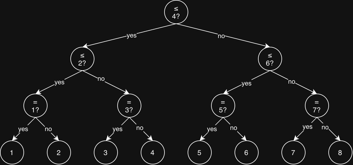
Compare an imbalanced decision tree that represents starting with the question "is it less than or equal to \(6\)?":
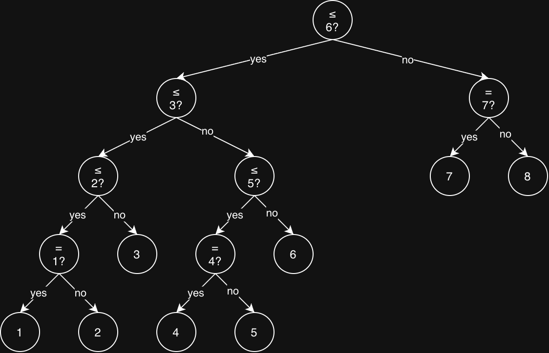
Note how the left subtree is deeper than the right subtree. If we get lucky and the answer to the first question is "no", it will take a total of only \(2\) questions. However, if we are unlucky and the answer to the first question is "yes", then it will take a total of \(4\) questions in the worst case. Thus, the balanced tree is better, since we must ask \(3\) questions in the worst case.
Computer scientists call this sort of procedure a binary search. Note that each question we ask cuts the decision tree in half.
The Mathematical Formula
What's the mathematical relationship between the number of options (\(8\) in this example) and the number of questions (\(3\) in this example)? In other words, how do you calculate the number of questions if you know the number of options?
Here's one way to think about it. You are familiar with the base-\(2\) exponential function \(2^k\) that represents powers of \(2\); for instance, when \(k=3\), \(2^3 = 2 \cdot 2 \cdot 2\). In our example, \(2^3 = 8\). Notice that each level of the binary decision tree doubles the number of nodes. So we ask: what power must we raise \(2\) to in order to get \(8\)? The mathematical operation that answers this question is called a (base-\(2\)) logarithm. When we write
\[\log_2(8) = 3\]
we mean \(2^3 = 8\).
Just as addition and subtraction are inverses (\(a + b - b = a\) and \(a - b + b = a\), so adding \(b\) and then subtracting \(b\) or vice versa gets us back where we started at \(a\)) and division and multiplication are inverses (\((a \cdot b) / b = a\) and \((a / b) \cdot b = a\), assuming \(b \ne 0\), so multiplying by \(b\) and then dividing by \(b\) or vice versa gets us back where we started at \(a\)), so also the base-\(2\) logarithm is the inverse of the base-\(2\) exponential: each "undoes" the other. Thus:
\[2^{\log_2(a)} = \log_2(2^a) = a.\]
Unfortunately, this is a little harder to see because the notation is different (it doesn't use "infix" notation like addition and subtraction where the operator is written between the numbers). You can read it this way: if we start with \(a\) and first compute \(\log_2(a)\) and then plug it into \(2^k\), we get \(2^{\log_2(a)}\) which equals \(a\); if we start with \(a\) and first compute \(2^a\) and then plug it into \(\log_2(x)\), we get \(\log_2(2^a)\) which equals \(a\). Either way, we get back where we started, namely, \(a\). Note that this is only well-defined when \(a \gt 0\) since there's no solution to the equation \(2^k = 0\) or \(2^k = -4\), etc.
Consider the following table:
| # Options | # Questions | Exponential | Logarithm |
|---|---|---|---|
| 1 | 0 | \(2^0 = 1\) | \(\log_2(1) = 0\) |
| 2 | 1 | \(2^1 = 2\) | \(\log_2(2) = 1\) |
| 4 | 2 | \(2^2 = 4\) | \(\log_2(4) = 2\) |
| 8 | 3 | \(2^3 = 8\) | \(\log_2(8) = 3\) |
| 16 | 4 | \(2^4 = 16\) | \(\log_2(16) = 4\) |
| 32 | 5 | \(2^5 = 32\) | \(\log_2(32) = 5\) |
Thus, we've answered our question; if we have \(n\) equally likely options, the number of "yes/no" questions required to guarantee that we determine the selected option is
\[\log_2(n).\]
We call this quantity entropy. We can think of it intuitively as a measure of uncertainty: the more questions we have to ask, the less certain we are.
Units of Measurement
The unit of measurement is called bits. The term "bit" is short for "binary digit", i.e., either a \(1\) or a \(0\), or, if you prefer, a "yes" (\(1\)) or a "no" \((0)\).
There are other units of measurement, too, just as we can choose meters or feet to measure distance. These other units of measurement correspond to different logarithm bases and thus to questions with a different number of answers. Thus, for instance, the base-\(10\) logarithm is another choice. There are formulas for converting between logarithms of different bases, so the choice of base is just a convention. We choose base \(2\) since it is convenient for the binary world of computing.
Non-Integer Measurements
In the example above, I chose \(8\) options since this is an integer power of \(2\) and the example is easy to follow. However, everything still works when the number isn't an integer power of \(2\). For instance, I could have chosen \(10\) numbers, and in that case,
\[\log_2(10) \approx 3.3219.\]
You might reasonably ask "how can we possibly ask \(3.3219\) yes/no questions?". Indeed, this is not possible! We would have to round up to \(4\) questions. However, with a larger number of choices, say \(10,000\), we compute \(\log_2(10,000) \approx 13.29\) and we would round up to \(14\) questions. As the number of options grows, the extra question becomes a tiny fraction of the total number of questions, so there is less and less "waste". Additionally, as I will soon discuss, we are typically interested in the average number of questions across multiple games; thus, if one game takes \(4\) questions and another takes \(5\) questions, the average is \(4.5\) questions. A non-integer number makes sense when we are talking about averages.
Considering Probability
Now, suppose that each number from \(1\) to \(8\) is equally likely, so each has probability of \(p=1/8\). More generally, for \(n\) choices, we have
\[p = \frac{1}{n}.\]
If we solve this equation for \(n\), we get:
\[n = \frac{1}{p}.\]
Thus, in the case that all options are equally likely, we can rewrite our formula for entropy in terms of probability:
\[\log_2(n) = \log_2\left(\frac{1}{p}\right).\]
Now, let's add a twist to our guessing game. Suppose that the options aren't all equally likely, that is, some options are more likely than others. Suppose we play our guessing game with four options, the letters \(A\), \(B\), \(C\), and \(D\), with the following probabilities:
- \(A\) - probability \(1/2 = 0.5\),
- \(B\) - probability \(1/4 = 0.25\),
- \(C\) - probability \(1/8 = 0.125\),
- \(D\) - probability \(1/8 = 0.125\).
Note that these values sum to \(1\), which is essential (the total probability must be 100%).
Distributions
We define a function \(p\) called a probability distribution that indicates the probabilities of each option:
- \(p(A) = 1/2\),
- \(p(B) = 1/4\),
- \(p(C) = 1/8\),
- \(p(D) = 1/8\).
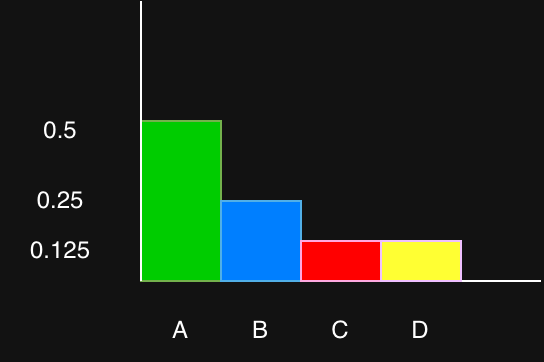
A distribution tells us how the values are distributed. Its key property is that the numbers add to \(1\) (i.e., 100%): the probability that the value will be \(A\), \(B\), \(C\), or \(D\) must be 100% since there are no other options (and it can't be more than this!). You can think of this distribution as a table:
| A | B | C | D |
|---|---|---|---|
| 0.5 | 0.25 | 0.125 | 0.125 |
You can visualize a distribution as a bar graph:
The Updated Game
As before, we play the following game: I've chosen a value according to these probabilities (half the time I choose \(A\), a quarter of the time \(B\), an eighth of the time \(C\), and an eighth of the time \(D\)). Now, if your goal is, as before, to guess my selection with as few "yes/no" questions as possible in a single game, then the probabilities actually don't matter at all: the best strategy is still a binary search. We can choose any two letters (let's just say \(B\) and \(D\)) and we then ask "is the letter \(B\) or \(D\)?". If the answer is "yes", we then ask "is it \(B\)?" and the answer determines the letter; if the answer is "no", we then ask "is it \(A\)?" and the answer determines the letter. We've just done a binary search again. We just split the options in half each time. In other words, we're interested in the worst case: I could pick the least likely option for a single game, so you have to prepare for the worst.
However, suppose we set a different goal: instead of doing our best for a single game, we try to do our best over multiple games. Here's an example to illustrate the difference between these two goals. Suppose we play \(8\) games. If we choose the strategy above ("is it \(B\) or \(D\)?"), then we must ask \(2 \cdot 8 = 16\) questions overall. Suppose instead that we choose the following strategy: first ask "is the letter \(A\)?", then ask "is the letter \(B\)?", then ask "is the letter \(C\)?"; in other words, we try to get as close to a split in half as possible:
- question 1 ("is it \(A\)?") splits exactly \(50/50\) since \(A\) has a 50% probability;
- question 2 ("is it \(B\)?") splits the odds of all remaining options (\(50\%\) total) into two equal \(25\%\) halves;
- question 3 ("is it \(C\)?") splits the odds of all remaining options \(25\%\) into two equal \(12.5\%\) halves.
The Decision Tree Method
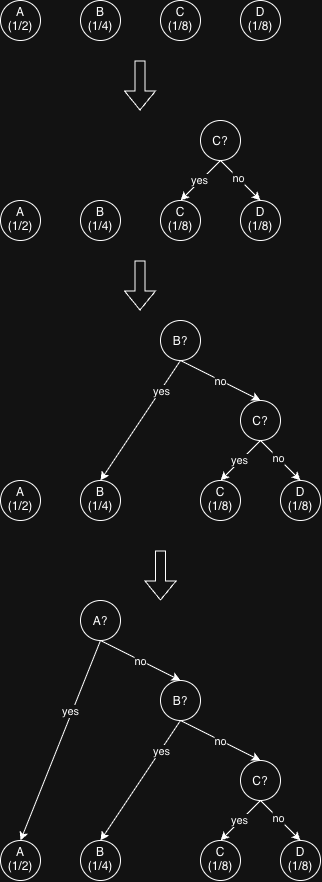
In this example it wasn't too hard to figure this out, but there's a procedure for determining this best split. We will maintain a list of decision trees. The probability of each tree is the sum of the probabilities of each of its leaf nodes.
- Create a tree for each option (here, \(A\), \(B\), \(C\), \(D\)). Each tree is just a single leaf node at this point.
- Select the two trees in the list with the lowest probabilities.
- Combine these trees into a new decision tree. The question the decision tree asks is: "is the secret value among any of the leaf nodes in my left subtree?".
- Repeat from step \(2\) until only one decision tree is left.
The following figure illustrates this procedure:
Expected Outcomes
We know the probabilities of each letter, so we expect the following results:
- in \(\frac{1}{2} \cdot 8 = 4\) games the letter is \(A\);
- in \(\frac{1}{4} \cdot 8 = 2\) games the letter is \(B\);
- in \(\frac{1}{8} \cdot 8 = 1\) game the letter is \(C\);
- in \(\frac{1}{8} \cdot 8 = 1\) game the letter is \(D\).
How many questions will we ask with our alternative strategy? Well:
- \(4\) times (when \(A\) is the secret letter) we will ask only \(1\) question ("is it \(A\)?"),
- \(2\) times (when \(B\) is the secret letter) we will ask \(2\) questions ("is it \(A\)?", "is it \(B\)?"),
- one time (when \(C\) is the secret letter) we will ask \(3\) questions ("is it \(A\)?", "is it \(B\)?", "is it \(C\)?"),
- and one time (when \(D\) is the secret letter) we will ask \(3\) questions ("is it \(A\)?", "is it \(B\)?", "is it \(C\)?", and the answer "no" to the last question reveals that \(D\) must be the secret letter).
This is a total of
\[4 \cdot 1 + 2 \cdot 2 + 1 \cdot 3 + 1 \cdot 3 = 14\]
questions. Notice that \(14 \lt 16\)!
Worst Case vs. Average Case
Thus, the strategy that works best for a single game is not the strategy that works best for multiple games! We can also express this fact by saying that the strategy that works best for a single game is optimized for the worst case whereas the strategy that works best for multiple games is optimized for the average case.
"Worst case" means that the probabilities don't matter; even if an option has a very small probability (say \(0.000001\%\)) it is possible that this choice could be made in a very unlikely scenario for any single game, so we have to treat it like all other options; our goal is to find a value, no matter how unlikely that value is. The most effective method is binary search.
"Average case" means that the probabilities are essential since they tell us the proportions of expected outcomes across multiple games; our goal is to prioritize in terms of probability. The most effective method is the decision tree method.
The following table summarizes the differences between the two strategies.
| Strategy | Method | Probabilities? | Trials |
|---|---|---|---|
| Worst Case | Binary Search | Don't Matter | Single Game |
| Average Case | Decision Tree | Essential | Multiple Games |
The Formula
What formula computes the total number of questions needed over multiple games? Note the following table:
| Secret Letter | Probability | # Questions | Formula |
|---|---|---|---|
| \(A\) | \(p(A)=\frac{1}{2}\) | \(1\) | \(\log_2\left(\frac{1}{p(A)}\right) = \log_2(2) = 1\) |
| \(B\) | \(p(B)=\frac{1}{4}\) | \(2\) | \(\log_2\left(\frac{1}{p(B)}\right) = \log_2(4) = 2\) |
| \(C\) | \(p(C)=\frac{1}{8}\) | \(3\) | \(\log_2\left(\frac{1}{p(C)}\right) = \log_2(8) = 3\) |
| \(D\) | \(p(D)=\frac{1}{8}\) | \(3\) | \(\log_2\left(\frac{1}{p(D)}\right) = \log_2(8) = 3\) |
Thus, the same formula happens to compute the number of questions needed, namely, for any letter \(L\):
\[\log_2\left(\frac{1}{p(L)}\right).\]
Averages
Recall the usual notion of the average of numbers: we add the numbers and divide by the count of numbers. So, for instance, the average of
\[1,1,2,2,2,3,3,4,4,4,4,6\]
is
\[\frac{1+1+2+2+2+3+3+4+4+4+4+6}{12} = 3.\]
Note that we can group the numbers like so:
\[\frac{(1+1) + (2+2+2) + (3+3) + (4+4+4+4) + 6}{12} = 3.\]
We can then factor these grouped sums as follows:
\[\frac{1 \cdot 2 + 2 \cdot 3 + 3 \cdot 2 + 4 \cdot 4 + 6 \cdot 1}{12}.\]
We can then break up the fraction as follows:
\[\frac{1 \cdot 2}{12} + \frac{2 \cdot 3}{12} +\frac{3 \cdot 2}{12} + \frac{4 \cdot 4}{12} + \frac{6 \cdot 1}{12}.\]
We can also write this as follows:
\[1 \cdot \frac{2}{12} + 2 \cdot \frac{3}{12} + 3 \cdot \frac{2}{12} + 4 \cdot \frac{4}{12} + 6 \cdot \frac{1}{12}.\]
Note that these fractions sum to \(1\):
\[\frac{2}{12} + \frac{3}{12} + \frac{2}{12} + \frac{4}{12} + \frac{1}{12} = 1.\]
Thus, they represent a probability distribution! The distribution is defined as follows:
- \(p(1) = 2/12\),
- \(p(2) = 3/12\),
- \(p(3) = 2/12\),
- \(p(4) = 4/12\),
- \(p(6) = 1/12\).
Thus, if we write the unique values in our list as follows
- \(x_1 = 1\),
- \(x_2 = 2\),
- \(x_3 = 3\),
- \(x_4 = 4\),
- \(x_5 = 6\),
then we can write the average of our list of numbers as follows (where \(n=5\) since there are \(5\) distinct numbers):
\[\sum_{i=1}^n x_i \cdot p(x_i).\]
Such a sum is sometimes called a weighted average or expected value.
Now we can express averages in terms of probabilities.
Entropy, Again
Remember that we determined that for an option \(x\) of probability \(p(x)\) the number of questions required in the optimal strategy is \(\log_2(1/p(x))\). Thus, the average number of questions needed is
\[\sum_{i=1}^n p(x_i) \cdot \log_2\left(\frac{1}{p(x_i)}\right).\]
This formula is called entropy.
Example
Let's use this formula to compute the number of questions required for \(8\) rounds of our \(4\)-letter guessing game. We have:
- \(x_1 = A\),
- \(x_2 = B\),
- \(x_3 = C\),
- \(x_4 = D\).
Then, since \(n=4\) (there are \(4\) options), we compute:
\begin{align*}\sum_{i=1}^4 p(x_i) \cdot \log_2(1/p(x_i)) &= p(x_1) \cdot \log_2(1/p(x_1)) + p(x_2) \cdot \log_2(1/p(x_2)) + p(x_3) \cdot \log_2(1/p(x_3)) + p(x_4) \cdot \log_2(1/p(x_4)) \\&= p(A) \cdot \log_2(1/p(A)) + p(B) \cdot \log_2(1/p(B)) + p(C) \cdot \log_2(1/p(C)) + p(D) \cdot \log_2(1/p(D)) \\&= \frac{1}{2} \cdot 1 + \frac{1}{4} \cdot 2 + \frac{1}{8} \cdot 3 + \frac{1}{8} \cdot 3 \\&= 3.\end{align*}
Thus, on average, \(3\) questions are needed.
Comparing Formulas
Let's return to our very first example: the guessing game involving \(8\) equally likely number options. Let's compute the entropy using our new formula:
\begin{align*}p(1) \cdot \log_2\left(\frac{1}{p(1)}\right) + \dots + p(8) \cdot \log_2\left(\frac{1}{p(8)}\right) &= \frac{1}{8} \cdot 3 + \dots + \frac{1}{8} \cdot 3 \\&= \frac{1}{8} \cdot 8 \cdot 3 \\&= 3 \\&= \log_2(8).\end{align*}
Now, remember our original formula for the worst-case situation; it tells us that, for a single game, the number of questions we must ask is:
\[\log_2(8).\]
Since we ask this many questions for every game, the average number of questions we would ask with this strategy over multiple games is also \(\log_2(8)\).
Thus, we computed the same result using the new formula and the old formula! We've thus discovered something: when every option is equally likely, the worst case strategy (averaged over multiple games) and the average case strategy (over multiple games) produce the same results.
Conditional Entropy
Next, we'll add yet another twist to our four-letter guessing game. As before, we will play multiple rounds of the game and our goal is to minimize the number of questions we must ask on average. However, now you will get a clue that reveals something about the secret letter.
In particular, I'll tell you whether the letter is a consonant or a vowel. Recall that we have the following distribution:
- \(p(A) = \frac{1}{2}\),
- \(p(B) = \frac{1}{4}\),
- \(p(C) = \frac{1}{8}\),
- \(p(D) = \frac{1}{8}\).
Since the consonants are \(B\), \(C\), and \(D\) and the only vowel is \(A\), we have the following probability distribution:
- \(p(\text{Consonant}) = p(B) + p(C) + p(D) = \frac{1}{4} + \frac{1}{8} + \frac{1}{8} = \frac{1}{2} = 0.5\);
- \(p(\text{Vowel}) = p(A) = \frac{1}{2} = 0.5\).
Let's calculate the entropy without any clue first:
\begin{align*}\sum_{i=1}^4 p(L_i) \cdot \log_2\left(\frac{1}{p(L_i)}\right) &= p(A) \cdot \log_2\left(\frac{1}{p(A)}\right) + p(B) \cdot \log_2\left(\frac{1}{p(B)}\right) + p(C) \cdot \log_2\left(\frac{1}{p(C)}\right) + p(D) \cdot \log_2\left(\frac{1}{p(D)}\right) \\&= \frac{1}{2} \cdot \log_2(2) + \frac{1}{4} \cdot \log_2(4) + \frac{1}{8} \cdot \log_2(8) + \frac{1}{8} \cdot \log_2(8) \\&= \frac{1}{2} \cdot 1 + \frac{1}{4} \cdot 2 + \frac{1}{8} \cdot 3 + \frac{1}{8} \cdot 3 \\&= 1\frac{3}{4} \\&= 1.75. \end{align*}
Suppose the clue is that the secret letter is a vowel. Well, then the letter must be \(A\) since it is the only vowel! Here's another way to think about this. First, we look at all the remaining options after the clue (there's only one in this case, namely, \(A\)). Then we try to make a new probability distribution for all the remaining options. Remember, the probabilities have to sum to \(1\) (100%). We do this by dividing the probabilities of the remaining options by the probability of the clue so that they now add up to \(1\) as follows:
\[p(A \mid \text{Vowel}) = \frac{p(A)}{p(\text{Vowel})} = \frac{0.5}{0.5} = 1.\]
Note that all of the other probabilities are \(0\) (e.g., \(p(B \mid \text{Vowel}) = 0\)).
Now suppose that the clue is that the secret letter is a consonant. The remaining options after this clue are then \(B\), \(C\), and \(D\). Let's apply our method to rescale the probabilities and make a new distribution:
- \(p(B \mid \text{Consonant}) = \frac{p(B)}{p(\text{Consonant})} = \frac{0.25}{0.5} = 0.5\),
- \(p(C \mid \text{Consonant}) = \frac{p(C)}{p(\text{Consonant})} = \frac{0.125}{0.5} = 0.25\),
- \(p(D \mid \text{Consonant}) = \frac{p(D)}{p(\text{Consonant})} = \frac{0.125}{0.5} = 0.25\).
Note that \(p(A \mid \text{Consonant}) = 0\).
These scaled probability distributions are called conditional probability distributions and the values are the conditional probabilities. You can read \(p(B \mid \text{Consonant})\), for instance, as "the probability of letter \(B\) given clue \(\text{Consonant}\)".
Now, how many questions do we need to ask on average after we receive the clue? Well, let's calculate the entropy using our formula, but let's use this new conditional distribution.
Suppose that the clue was that the secret letter is a vowel. We compute the following:
\begin{align*}p(A \mid \text{Vowel}) \cdot \log_2\left(\frac{1}{p(A \mid \text{Vowel})}\right) &= 1 \cdot \log_2(1) \\&= 1 \cdot 0 \\&= 0.\end{align*}
In this case there is no entropy whatsoever because the outcome is certain!
Suppose the clue was that the secret letter is a consonant. We compute the following:
\begin{align*}p(B \mid \text{Consonant}) \cdot \log_2\left(\frac{1}{p(B \mid \text{Consonant})}\right) &+ p(C \mid \text{Consonant}) \cdot \log_2\left(\frac{1}{p(C \mid \text{Consonant})}\right) \\&+ p(D \mid \text{Consonant}) \cdot \log_2\left(\frac{1}{p(D \mid \text{Consonant})}\right) \\&= \frac{1}{2} \cdot \log_2(2) + \frac{1}{4} \cdot \log_2(4) + \frac{1}{4} \cdot \log_2(4) \\&= 1\frac{1}{2} \\&= 1.5\end{align*}
We can write this as follows (where in our case \(n=4\) and \(x_i\) represents each letter individually and \(y_j\) represents a single clue):
\[\sum_{i=1}^n p(x_i \mid y_j) \cdot \log_2\left(\frac{1}{p(x_i \mid y_j)}\right).\]
Note that we implicitly exclude any values where \(p(x_i \mid y_j) = 0\) since \(\log_2(0)\) is undefined. That's why we skipped the \(p(A \mid \text{Consonant})\) case in the sum above.
This just computes the entropy in one case, i.e., for a particular clue. We want to compute the average entropy over all the clues. We already know how to compute averages though! We just apply our formula from earlier to average all these values:
\[\sum_{j=1}^m p(y_j) \cdot \sum_{i=1}^n p(x_i \mid y_j) \cdot \log_2\left(\frac{1}{p(x_i \mid y_j)}\right).\]
In our example, we thus compute:
\begin{align*}p(\text{Vowel}) \cdot 0 + p(\text{Consonant}) \cdot 1.5 \\&= 0.5 \cdot 0 + 0.5 \cdot 1.5 \\&= 0.75.\end{align*}
Thus, we can compute the conditional entropy, i.e., the average entropy given clues.
Now, let's consider the following: we started with entropy \(1.75\) and ended with entropy \(0.75\). This is a difference of \(1.75 - 0.75 = 1.0\) bits of entropy. That means that we removed \(1.0\) bit of entropy (or that we saved \(1\) question on average).
We call this measure of the entropy removed mutual information.
Cryptography
Let's now apply our knowledge of information theory to analyze cryptographic ciphers!
A cipher is an algorithm that converts a plaintext (legible source text) into a ciphertext (secret text).
Let's consider a few examples of ciphers.
Caesar Cipher
The Caesar cipher "rotates" each letter by a fixed number of positions in the alphabet. It is named after Julius Caesar, who reportedly used this cipher. Each letter is assigned a position, where \(A=0\), \(B=1\), \(C=2\), etc., and \(Z=25\). Consider the following figure:
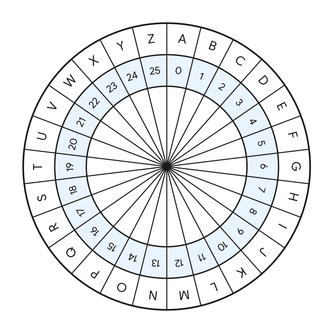
A shift of \(1\) would map \(A\) to \(B\), \(C\) to \(D\), \(Z\) to \(A\), etc. A shift of \(13\) would map \(A\) to \(N\), \(X\) to \(K\), etc. This is computed as follows for a letter \(l\):
\[\mathrm{letter}((\mathrm{position}(l) + s) \bmod 26).\]
Here, \(\mathrm{letter}\) maps a position to a letter (e.g., \(\mathrm{letter}(0) = A\)) and \(\mathrm{position}\) maps a letter to a position (e.g., \(\mathrm{position}(A) = 0\)). The variable \(s\) represents the shift amount, and \(\bmod 26\) is division modulo \(26\), i.e., the remainder after dividing by \(26\) (e.g., \(36 \bmod 26 = 10\)). The modular arithmetic is what makes the shift "circular" - it makes the positions "wrap around" once they exceed the maximum position.
Thus, for the plaintext
\[\texttt{ALICE WAS BEGINNING TO GET VERY TIRED}\]
the cipher text with a shift of \(15\) would be
\[\texttt{PAXRT LPH QTVXCCXCV ID VTI KTGN IXGTS}.\]
Intuitively, the Caesar cipher is weak - once we figure out any letter, we've figured out every letter.
Vigenère Cipher
The Vigenère cipher is like the Caesar cipher, except that it uses different shifts for each letter. It does so by specifying a key, which is any sequence of letters. For instance, we could specify the key "WONDERLAND". The letter "W" indicates a shift of \(22\), the letter "O" indicates a shift of \(14\), etc. If we have the plaintext
\[\texttt{ALICE WAS BEGINNING TO GET VERY TIRED},\]
we would repeat the key until it matches the length of the message, for instance
\[\texttt{WONDE RLA NDWONDERL AN DER LAND WONDER}.\]
We truncate the key once we reach the required number of letters. The ciphertext in this example is:
\[\texttt{WZVFI NLS OHCWAQMER TB JAH IHVP EIEHZ}.\]
Thus, the formula for the \(i\)-th letter \(l_i\) in our plaintext and \(i\)-th letter \(k_i\) in our key (which has length \(K\)) is
\[\mathrm{letter}((\mathrm{position}(l_i) + \mathrm{position}(k_{i \bmod K})) \bmod 26).\]
Intuitively, the Vigenère cipher is better than the Caesar cipher (which is just the Vigenère cipher with a single-letter key). Once we exhaust all the letters in the key we start repeating ourselves, and intuitively this reveals information.
One-Time Pad
The one-time pad is like the Vigenère cipher, except for the following differences:
- It uses a truly random key (that is, not a pseudo-random key); computers can generate pseudo-random numbers with various algorithms; this requires truly random numbers, which can be drawn from sources of randomness in nature.
- The key must be at least as long as the plaintext message;
- The key can never be re-used (i.e., once we're ciphered one message, we must "throw it away").
This is the only encryption method proved to be theoretically unbreakable!
Analyzing Ciphers
Let's figure out how to analyze these ciphers using a "guessing game" as before.
First, let's start with the following game.
First, I know the distribution \(p(l)\) of letters \(l\) in the plaintext message: I just count how many times a letter occurs in the message and then divide by the length of the message. For instance, in
\[\texttt{ALICE WAS BEGINNING TO GET VERY TIRED},\]
\(p(G) = \frac{3}{31}\). Note that spaces aren't part of the message; we just write them for legibility. The message is just a sequence of capital letters.
Now, I draw letters at random in proportion to this distribution (e.g., \(3/31\) of the time I draw \(G\)). This is just our usual game: each letter isn't equally likely.
Now, there's a slight twist: I also draw a key at random. No key is more likely than the others, so every key has equal probability. For instance, in the Caesar cipher, there are 26 possible keys, so each key has probability \(1/26\). In the Vigenère Cipher with a key of length \(2\), there are \(26 \cdot 26\) possibilities, so each key has probability \(1/26^2\). In general, for a key of length \(n\), each key has probability \(1/26^n\).
I then encrypt the letter using the cipher and the key. The "clue" I give you is the encrypted letter. Your goal is to guess the plaintext letter given this clue by asking "yes/no" questions. How many "yes/no" questions are required on average?
Let's use our formula!
Joint Distributions
Before we start plugging in values, there's a small catch: our old formula for conditional probability won't work in this case, i.e., we can't just use
\[p(P \mid C) = \frac{p(P)}{p(C)}.\]
Why not? In our previous example with consonants and vowels, each letter corresponded to a unique clue (a letter is either a consonant or a vowel but not both). However, plaintext letters can map to multiple clues, since we can choose different keys (and indeed, in most ciphers, the mapping isn't constant even for a fixed key).
To solve this issue, we use a new tool called a joint distribution. This is just a "two-dimensional" distribution. You can think of it as a grid of numbers.
For instance, the joint distribution for our old vowel and consonant example looks like this:
| Vowel | Consonant | |
|---|---|---|
| A | 1/2 | 0 |
| B | 0 | 1/4 |
| C | 0 | 1/8 |
| D | 0 | 1/8 |
The value \(p(l, c)\) tells us how likely it is that letter \(l\) corresponds to clue \(c\). Where did the number come from? Well, recall that \(p(A) = 1/2\). In the joint distribution, we "spread out" this probability across each of the columns. How often does \(A\) correspond to a vowel? Well, 100% of the time! So we put 100% of \(1/2\) in the vowel column. How often does \(A\) correspond to a consonant? Well, 0% of the time! So we put 0% of \(1/2\) in the consonant column. Similarly, we get \(0\) in the vowel column and 100% of the respective probability in the consonant column for letters \(B\), \(C\) and \(D\). Thus, in this example, notice that, in each row, there is exactly one non-zero column. So, this example is a special case.
Notice something else that's important: if we sum all the values in a row, we get the probability for the respective letter! Thus, for example, \(p(A) = p(A,\text{Vowel}) + p(A,\text{Consonant}) = 1/2\). Likewise, if we sum all the values in a column, we get the probability for the respective clue! Thus, for example, \(p(\text{Consonant}) = p(A, \text{Consonant}) + p(B, \text{Consonant}) + p(C, \text{Consonant}) + p(D, \text{Consonant}) = 1/2\).
Conditional Probability Amended
Thus, we amend our earlier formula for conditional probability as follows:
\[p(l \mid c) = \frac{p(l,c)}{p(c)}.\]
In the consonant and vowel example, it happened that \(p(l,c) = p(l)\), which is why our old formula worked.
The Single-Letter Game Analyzed
Let's return to the cipher game. The joint distribution \(p(l,c)\) tells us how likely it is that letter \(l\) corresponds to clue \(c\). How do we compute this? Well, we have a cipher that takes a letter and a key and encrypts it to a ciphered letter:
\[E(k, l) = c.\]
We then ask: which keys map the letter \(l\) to the clue \(c\), i.e., which keys \(k\) satisfy \(E(k, l) = c\)? Well, suppose that the answer is key \(k_1\) and key \(k_2\). We know the probability of these keys \(p(k_1)\) and \(p(k_2)\). We know the probability \(p(l)\) of letter \(l\). How much of probability \(p(l)\) do we distribute to "slot" \(p(l,c)\)? We must put \(p(l) \cdot (p(k_1) + p(k_2))\). Thus, in general, we have
\[p(l, c) = p(l) \cdot \sum_{k, E(k, l) = c} p(k).\]
Let's try to compute \(p(l,c)\) for our ciphers.
For the Caesar cipher, there are exactly \(26\) keys, one for each shift. There is exactly one key \(k\) that shifts \(l\) to \(c\), so we have
\[p(l,c) = p(l) \cdot \frac{1}{26}.\]
For the Vigenère cipher with a key of length \(2\) there are exactly \(26^2\) keys, one for each pair of shifts. Only the first one actually applies to the letter \(l\), though, so there are \(26\) key pairs \((k_1, k_2)\) that map to \(l\), so the overall odds are \(26/26^2 = 1/26\), so we have
\[p(l,c) = p(l) \cdot \frac{1}{26}.\]
Thus, the odds are exactly the same! In fact, we have the same odds for the one-time pad too! If we plug in these values to our formula for conditional probability, we'll get the same probability \(p(l \mid c)\) for all ciphers, and so we'll also get the same entropy and mutual information! Thus, the single-letter analysis doesn't tell us anything useful at all!
N-Gram Analysis
The solution is to analyze entire sequences of letters, not just single letters. These sequences of letters are called \(n\)-grams. A single letter is a \(1\)-gram, two letters is a \(2\)-gram, etc.
Let's describe the multiple-letter game.
First, I know the distribution of \(n\)-grams in the plaintext message. I just "slide" a "window" of length \(n\) over the text, like so:
\begin{align*}\mathtt{\boxed{\mathtt{ALICE}}WASBEGINNINGTOGETVERYTIRED} &\rightarrow \mathtt{A\boxed{\mathtt{LICEW}}ASBEGINNINGTOGETVERYTIRED} \\&\rightarrow \mathtt{AL\boxed{\mathtt{ICEWA}}SBEGINNINGTOGETVERYTIRED} \\&\rightarrow \mathtt{ALI\boxed{\mathtt{CEWAS}}BEGINNINGTOGETVERYTIRED} \\&\rightarrow \dots.\end{align*}
The example above shows the sliding window for \(5\)-grams. I then count how many times each \(n\)-gram occurs. I then divide all the counts by the total number of \(n\)-gram windows.
Now, I draw \(n\)-grams \(g\) from the plaintext message at random in proportion to this distribution. I also draw a key \(k\) at random (and each key is equally likely).
Then, I encrypt \(E(k, g) = c\) and give you the clue \(c\) (the encrypted \(n\)-gram, which is itself an \(n\)-gram). Your goal is to guess the \(n\)-gram by asking "yes/no" questions. How many questions will it take on average?
Well, our formula for conditional entropy answers this!
\[\sum_c p(c) \cdot \sum_g p(g \mid c) \cdot \log_2\left(\frac{1}{p(g \mid c)}\right).\]
We can compute \(p(g \mid c)\) using our formula from before:
\[p(g \mid c) = \frac{p(g,c)}{p(c)}.\]
We can compute \(p(g,c)\) just as before:
\[p(g,c) = p(g) \cdot \sum_{k,E(k,g) = c} p(k).\]
Thus, we have all the ingredients we need to analyze these ciphers! Our hypothesis is that the Caesar cipher is the "weakest" cipher, the Vigenère cipher is stronger, and the one-time pad is the strongest. But how do we measure this "strength"? We use entropy and mutual information!
At this point, the calculations will become extremely tedious. It's better to have a computer do them. So, let's write some code!
Python Code
Let's write some Python code that can analyze these ciphers!
Remember that we need to know the distribution of \(n\)-grams for the plaintext message, so let's write a function to get the \(n\)-gram distribution of the plaintext message.
def get_plain_distribution(text, n):
  ...
Here are some hints:
- The
ordfunction takes a character and returns its Unicode code point (a number that represents that character). For instance:ord("A") = 65.ordabbreviates the word "ordinal". - We will only use capital letters just to simplify things.
- We won't use the characters (letters) themselves; instead, we'll map \(A\) to \(0\), \(B\) to \(1\), \(Z\) to 25, etc. In other words, we will work with each letter's index instead of the letter itself. It will be easier this way.
- You can subtract
ord("A")from a letter's code point to get the letter's index since Unicode encodes the capital letters in sequence (\(A\) is \(65\), \(B\) is \(66\), etc.). For instance, sinceord("B") = 66, you can compute its index (which should be \(1\)) by subtractingord("A")since \(66-65=1\), etc. - I recommend that you use Python list comprehensions.
- Write a list comprehension that computes the index for every letter in the text.
- Capitalize the text before you process it.
- Only include letters between A and Z. Don't include spaces or punctuation, etc.
- Write a list comprehension that computes the \(n\)-grams.
- The
tuplefunction takes a list like[1,2,3,4,5]and makes a tuple like(1,2,3,4,5). - You can make a "slice" of a list with the syntax
my_list[start : end]. This will be useful for implementing the "sliding window". - The
rangefunction creates a range from `0..m (where \(m\) is an exclusive index) that you can iterate over.
- The
- Write a list comprehension that computes the index for every letter in the text.
- Use
Counterfrom thecollectionspackage. It creates a sparse histogram. It can count the \(n\)-grams. - Return a dictionary that maps each \(n\)-gram to its probability, i.e., its count divided by the total number of values in the
Counter. This represents the probability distribution. You can use comprehensions with dictionaries too. In fact, you can use comprehensions with many different constructs in Python.
def get_plain_distribution(text, n):
  # (1) compute the indices of all letters in the text
  # letters = ...
  # (2) compute the n-grams by sliding a window over the indices
  # ngrams = ...
  # (3) create a Counter initialized with the ngrams
  # counts = ...
  # (4) sum the total count
  # total = ...
  # (5) return the distribution as a dictionary
  # return ...
Try to write it yourself. Here is one solution:
def get_plain_distribution(text, n):
    letters = [ord(letter) - ord("A") for letter in text.upper() if "A" <= letter <= "Z"]
    ngrams = [tuple(letters[i : i + n]) for i in range(len(letters) - n +1)]
    counts = Counter(ngrams)
    total = sum(counts.values())
    return { gram: count / total for gram, count in counts.items() }
Let's run this on some sample text:
MESSAGE= """
Alice was beginning to get very tired
"""

print(get_plain_distribution(MESSAGE, 2))
The result is:
{(0, 11): 0.03333333333333333, (11, 8): 0.03333333333333333, (8, 2): 0.03333333333333333, (2, 4): 0.03333333333333333, (4, 22): 0.03333333333333333, (22, 0): 0.03333333333333333, (0, 18): 0.03333333333333333, (18, 1): 0.03333333333333333, (1, 4): 0.03333333333333333, (4, 6): 0.03333333333333333, (6, 8): 0.03333333333333333, (8, 13): 0.06666666666666667, (13, 13): 0.03333333333333333, (13, 8): 0.03333333333333333, (13, 6): 0.03333333333333333, (6, 19): 0.03333333333333333, (19, 14): 0.03333333333333333, (14, 6): 0.03333333333333333, (6, 4): 0.03333333333333333, (4, 19): 0.03333333333333333, (19, 21): 0.03333333333333333, (21, 4): 0.03333333333333333, (4, 17): 0.03333333333333333, (17, 24): 0.03333333333333333, (24, 19): 0.03333333333333333, (19, 8): 0.03333333333333333, (8, 17): 0.03333333333333333, (17, 4): 0.03333333333333333, (4, 3): 0.03333333333333333}The tuple (0,11) represents the \(2\)-gram AL for instance; it was assigned probability 0.033....
Next, let's create a function that computes the (unconditional) entropy of a distribution, i.e.,
\[\sum_x p(x) \cdot \log_2\left(\frac{1}{p(x)}\right).\]
def entropy(distribution):
  ...
Try to write it yourself. Here's one solution:
def entropy(distribution):
    return sum(p * math.log2(1.0 / p) for p in distribution.values())
Next, we need to compute every possible key for each cipher. Let's start with the Caesar cipher.
Hints:
- Use a list comprehension.
- If you write
(k,) * n, Python will create a tuple with \(n\) copies of \(k\), e.g.(2,) * 4 = (2,2,2,2).
def caesar_cipher(n):
  ...
Try to write it yourself. Here's one solution:
def caesar_keys(n):
    return [(k,) * n for k in range(26)]
Next, let's compute the keys for the one-time pad cipher.
def otp_keys(n):
  ...
Hints:
- Use the
itertools.productfunction and convert the result to a list using thelistfunction. Theitertools.productfunction creates every possible \(n\)-tuple within a given range.
Try it yourself. Here's one solution:
def otp_keys(n):
    return list(itertools.product(range(26), repeat=n))
Let's write a function to compute all possible keys for the Vigenère cipher. This one is a bit trickier.
Hint:
- It's very similar to the solution for the one-time pad cipher, except that, when the window size is longer than the Vigenère key length, we have to start repeating values.
- Use the modulus operator
%that computes the remainder after integer division to implement the repeating behavior.
def vigenere_keys(n, key_len):
  ...
Try to write it yourself. Here's one solution:
def vigenere_keys(n, key_len):
    return [
        tuple(base_key[i % key_len] for i in range(n))
        for base_key in itertools.product(range(26), repeat=key_len)
    ]
Let's write a function that applies a cipher given a plaintext \(n\)-gram and a key:
def cipher(p, k):
  ...
Try to write it yourself. Here's one solution:
def cipher(p, k):
    return tuple((p[i] + k[i]) % 26 for i in range(len(p)))
Next, let's write a function to compute the joint distribution. While we're at it, it will be convenient to compute the marginal distribution for the ciphertext at the same time.
def get_joint_and_cipher_distributions(plain_dist, keys):
  ...
  return joint_dist, cipher_dist
Recall that the formula for the joint distribution is
\[p(P, C) = p(P) \cdot \sum_{k, E(k, P) = C} p(k)\]
and the formula for the marginal distribution is
\[p(C) = \sum_P p(P, C).\]
Try to write it yourself. Hints:
- Use a
Counterfor each distribution. - We can compute these distributions in a single loop over the plaintext distribution items.
Here's one solution:
def get_joint_and_cipher_distributions(plain_dist, keys):
    key_prob = 1.0 / len(keys)
    joint_dist = Counter()
    cipher_dist = Counter()

    for p, p_prob in plain_dist.items():
        for k in keys:
            c = cipher(p, k)
            pc_prob = p_prob * key_prob
            joint_dist[(p, c)] += pc_prob
            cipher_dist[c] += pc_prob

    return joint_dist, cipher_dist
Next, let's write a function conditional_entropy that computes the condition entropy.
def conditional_entropy(plain_dist, joint_dist, cipher_dist):
  ...
Recall that the formula is
\[\sum_C p(C) \cdot H_C(P)\]
where
\[H_C(P) = \sum_P p(P \mid C) \cdot \log_2\left(\frac{1}{p(P \mid C)}\right).\]
Try to write it yourself. Hints:
- You can reuse the
entropyfunction if you compute a distribution corresponding to \(H_C(P)\). Just put the right values into a dictionary.
Here's one solution:
def conditional_entropy(plain_dist, joint_dist, cipher_dist):
    h_p_given_c = 0.0
    for c, c_prob in cipher_dist.items():
        cond_dist = {
            p: joint_dist[(p, c)] / c_prob
            for p in plain_dist
            if (p, c) in joint_dist
        }
        h_p_given_c += c_prob * entropy(cond_dist)

    return h_p_given_c
Next, let's write a function evalulate_cipher that computes 3 quantities: the entropy of the plaintext distribution, the conditional entropy of the plaintext distribution given the ciphertext distribution, and the mutual information. This function should accept the plaintext \(n\)-gram probability distribution and the list of all possible keys for the cipher:
def evaluate_cipher(plain_dist, keys):
    joint_dist, cipher_dist = get_joint_and_cipher_distributions(plain_dist, keys)
    h_p_given_c = conditional_entropy(plain_dist, joint_dist, cipher_dist)
    h_p = entropy(plain_dist)
    mutual_info = h_p - h_p_given_c
    return h_p, h_p_given_c, mutual_info
The complete program looks like this (where I've added a script at the end to print the results):
from collections import Counter
import math
import itertools

MESSAGE = """
Alice was beginning to get very tired of sitting by her sister on the bank,
and of having nothing to do: once or twice she had peeped into the book her sister was reading,
but it had no pictures or conversations in it, “and what is the use of a book,”
thought Alice “without pictures or conversations?”

So she was considering in her own mind (as well as she could,
for the hot day made her feel very sleepy and stupid), whether the pleasure of making
a daisy-chain would be worth the trouble of getting up and picking the daisies,
when suddenly a White Rabbit with pink eyes ran close by her.
"""

MAX_WINDOW_SIZE=3

def get_plain_distribution(text, n):
    letters = [ord(letter) - ord("A") for letter in text.upper() if "A" <= letter <= "Z"]
    ngrams = [tuple(letters[i : i + n]) for i in range(len(letters) - n +1)]
    counts = Counter(ngrams)
    total = sum(counts.values())
    return { gram: count / total for gram, count in counts.items() }

def entropy(distribution):
    return sum(p * math.log2(1.0 / p) for p in distribution.values())

def caesar_keys(n):
    return [(k,) * n for k in range(26)]

def vigenere_keys(n, key_len):
    return [
        tuple(base_key[i % key_len] for i in range(n))
        for base_key in itertools.product(range(26), repeat=key_len)
    ]

def otp_keys(n: int) -> list[tuple[int, ...]]:
    return list(itertools.product(range(26), repeat=n))

def cipher(p, k):
    return tuple((p[i] + k[i]) % 26 for i in range(len(p)))

def get_joint_and_cipher_distributions(plain_dist, keys):
    key_prob = 1.0 / len(keys)
    joint_dist = Counter()
    cipher_dist = Counter()

    for p, p_prob in plain_dist.items():
        for k in keys:
            c = cipher(p, k)
            pc_prob = p_prob * key_prob
            joint_dist[(p, c)] += pc_prob
            cipher_dist[c] += pc_prob

    return joint_dist, cipher_dist

def conditional_entropy(plain_dist, joint_dist, cipher_dist):
    h_p_given_c = 0.0
    for c, c_prob in cipher_dist.items():
        cond_dist = {
            p: joint_dist[(p, c)] / c_prob
            for p in plain_dist
            if (p, c) in joint_dist
        }
        h_p_given_c += c_prob * entropy(cond_dist)

    return h_p_given_c

def evaluate_cipher(plain_dist, keys):
    joint_dist, cipher_dist = get_joint_and_cipher_distributions(plain_dist, keys)
    h_p_given_c = conditional_entropy(plain_dist, joint_dist, cipher_dist)
    h_p = entropy(plain_dist)
    mutual_info = h_p - h_p_given_c
    return h_p, h_p_given_c, mutual_info

for n in range(1, MAX_WINDOW_SIZE+1):
        plain_dist = get_plain_distribution(MESSAGE, n=n)
        print(f"=== Window size n = {n} ===")
        for name, keys in [
            ("Caesar (key length 1)", caesar_keys(n)),
            ("Vigenere (key length 2)", vigenere_keys(n, key_len=2)),
            ("One-Time Pad (key length n)", otp_keys(n)),
        ]:
            h_p, h_p_given_c, mi = evaluate_cipher(plain_dist, keys)
            print(
                f"  {name:27s} | H(P) = {h_p:.4f} | "
                f"H(P|C) = {h_p_given_c:.4f} | I(P;C) = {mi:z.4f} bits"
            )
        print()
Here's the output:
=== Window size n = 1 ===
  Caesar (key length 1)       | H(P) = 4.1378 | H(P|C) = 4.1378 | I(P;C) = 0.0000 bits
  Vigenere (key length 2)     | H(P) = 4.1378 | H(P|C) = 4.1378 | I(P;C) = 0.0000 bits
  One-Time Pad (key length n) | H(P) = 4.1378 | H(P|C) = 4.1378 | I(P;C) = 0.0000 bits

=== Window size n = 2 ===
  Caesar (key length 1)       | H(P) = 7.0911 | H(P|C) = 2.5083 | I(P;C) = 4.5827 bits
  Vigenere (key length 2)     | H(P) = 7.0911 | H(P|C) = 7.0911 | I(P;C) = 0.0000 bits
  One-Time Pad (key length n) | H(P) = 7.0911 | H(P|C) = 7.0911 | I(P;C) = 0.0000 bits

=== Window size n = 3 ===
  Caesar (key length 1)       | H(P) = 8.2687 | H(P|C) = 0.4266 | I(P;C) = 7.8422 bits
  Vigenere (key length 2)     | H(P) = 8.2687 | H(P|C) = 3.6609 | I(P;C) = 4.6078 bits
  One-Time Pad (key length n) | H(P) = 8.2687 | H(P|C) = 8.2687 | I(P;C) = 0.0000 bits
Results
Here are the results in tables:
Window Size n = 1
| Cipher | Key Length | Message Entropy | Conditional Entropy | Mutual Information |
|---|---|---|---|---|
| Caesar | 1 | 4.1378 bits | 4.1378 bits | 0 bits |
| Vigenère | 2 | 4.1378 bits | 4.1378 bits | 0 bits |
| One-Time Pad | n | 4.1378 bits | 4.1378 bits | 0 bits |
Window Size n = 2
| Cipher | Key Length | Message Entropy | Conditional Entropy | Mutual Information |
|---|---|---|---|---|
| Caesar | 1 | 7.0911 bits | 2.5083 bits | 4.5827 bits |
| Vigenère | 2 | 7.0911 bits | 7.0911 bits | 0 bits |
| One-Time Pad | n | 7.0911 bits | 7.0911 bits | 0 bits |
Window Size n = 3
| Cipher | Key Length | Message Entropy | Conditional Entropy | Mutual Information |
|---|---|---|---|---|
| Caesar | 1 | 8.2687 bits | 0.4266 bits | 7.8422 bits |
| Vigenère | 2 | 8.2687 bits | 3.6609 bits | 4.6078 bits |
| One-Time Pad | n | 8.2687 bits | 8.2687 bits | 0 bits |
These results demonstrate the following findings:
- A window size of \(1\) is insufficient to distinguish the ciphers (as we already figured out previously).
- The Vigenère cipher and the one-time pad cipher perform identically until the window size surpasses the Vigenère key size.
- The one-time pad consistently has \(0\) bits of mutual information (i.e., it never "leaks" information).
- The conditional entropy of the Vigenère cipher increases until the window size surpasses the key size and then it decreases.
- The conditional entropy of the one-time pad consistently increases as the window size increases.
Thus, we can define the relative strength of ciphers as follows: if there exists a window size such that the entropy of cipher A is greater than the entropy of cipher B and the mutual information of cipher A is lower than the mutual information of cipher B, then cipher A is stronger than cipher B. We can thus establish that
\[\text{Caesar} \lt \text{Vigenère} \lt \text{One-Time Pad}.\]
In fact, Claude Shannon proved that the one-time pad cipher is unbreakable (given the conditions listed for it). In fact, it is the only known cipher with this property. Why doesn't everyone use it then? Well, it is somewhat impractical for the following reasons:
- It requires true randomness for key generation, not pseudo-randomness that computers typically use.
- It requires the key length to be at least as long as the message length. This means that there has to be a maximum size for messages in practice.
- Each key can only be used once.
- The keys have to be communicated securely between parties and they'd have to agree in advance somehow about which keys they are using.
Nonetheless, it is possible to use OTP in practice. You might wonder how any cipher can be truly unbreakable, even with an infinite amount of time and computer power. Well, it is unbreakable because no decrypted message is more likely than any other. For instance, consider a 5-letter message like "APPLE". Every decryption is equally likely, so it is not possible to tell whether the original message was "APPLE" or "EARTH", or "BEACH", or "CHAIR", etc. Thus, even though it might be possible to "decrypt" the message, we would have maximum uncertainty about which of these potential "decryptions" is the right one!
Notes
Here are a few notes about the results:
- The window size must be small relative to the message size for this method to work effectively. Consider the extreme case when the window size equals the message size; the plaintext distribution would have only one entry with 100% probability.
- The window acts like a "probe" that we can use to test our texts; with a large enough window size, it has enough "memory" or "context" to distinguish ciphers.
- It isn't really possible to know the distribution of \(n\)-grams in the English language since there is no fixed corpus (people are writing new texts every day). However, sometimes, researchers will use a very large corpus of text to serve as a model for such an idealized distribution. We are using the plaintext message to compute a rough empirical distribution of \(n\)-grams.
Conclusion
We have thus validated our basic hypothesis: information theory gives us concrete metrics for evaluating the relative strength of ciphers.