Harmonic Oscillators

Imagine a spring suspended vertically downward from a horizontal surface with an object attached to the bottom of the spring, as in the following figure.

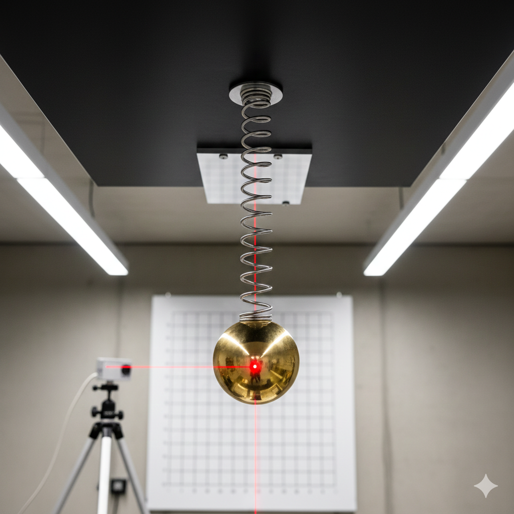
Suppose that both the spring and object are at rest (i.e., at equilibrium). We will denote the vertical position (height) of the object by \(x\), and we define the equilibrium position as \(x=0\). Suppose that we displace the object by some distance \(d\) at time \(t=0\). Treating \(x\) as a function of time, this means that \(x(0) = d\). We then release the object. How will the object move?

In our example, we will designate an upward displacement as positive (e.g., \(d = +1\)) and a downward displacement as negative (e.g., \(d = -1\)) though it does not matter as long as we are consistent.

In this simple scenario, the only force we consider is the restorative force \(F_r\) of the spring acting on the object to return it to its equilibrium position \(x=0\). If we push the spring upward, the restorative force will be downward, and if we pull the spring downward, the restorative force will the upward, i.e., the restorative force is opposite the displacement.

Hooke's law indicates that the restorative force is directly proportional and opposite to the displacement, i.e., for some constant or proportionality \(k > 0\),

\[F_r(t) = -k \cdot x(t).\]

Newton's second law of motion indicates that the force \(F_o\) acting upon the object is equal to the product of the (inertial) mass of the object and the acceleration of the object, i.e.,

\[F_o(t) = m \cdot a(t).\]

In this simplified model, we also neglect the mass of the spring itself.

The acceleration is the second derivative of position with respect to time, i.e., \(a = \ddot{x}(t)\). Thus, this may be written as

\[F_o(t) = m \cdot \ddot{x}(t).\]

Since the only force acting on the mass is the restorative force exerted by the spring, Newton's second law of motion indicates that

\[F_o = F_r,\]

i.e., that

\[m \cdot \ddot{x}(t) = -k \cdot x(t),\]

which is equivalent to

\[m \cdot \ddot{x}(t) + k \cdot x(t) = 0.\]

We assume that the initial velocity of the object is \(0\), i.e., that \(\dot{x}(0) = 0\). We then have a differential equation

\[m \cdot \ddot{x} + k \cdot x = 0\]

with two initial conditions:

• \(x(0) = d\), and
• \(\dot{x}(0) = 0\).

To determine the equation of motion, we must solve this differential equation to determine the function \(x\).

Recall that the exponential function \(\exp\) is defined as a fixed point of differentiation, i.e., \(\exp(0) = 1\) and \(\exp' = \exp\) and that \(\exp(t) = e^t\) where \(e\) is Euler's constant. This makes it extremely useful for solving certain ordinary differential equations. Substituting \(e^{rt}\) (where \(r \in \mathbb{C}\) is an arbitrary complex number) for \(x\) in the differential equation, we obtain

\[m \cdot \ddot{e^{rt}} + k \cdot e^{rt} = 0\]

which, since \(\dot{e^{rt}} = r \cdot e^{rt}\) by the chain rule and thus \(\ddot{e^{rt}} = r^2 \cdot e^{rt}\) by the product rule and a further application of the chain rule, is equivalent to

\[m \cdot r^2 \cdot e^{rt} + k \cdot e^{rt} = 0.\]

This means that

\[e^{rt} \cdot (m \cdot r^2 + k) = 0\]

which is satisfied if and only if the characteristic equation

\[m \cdot r^2 + k = 0\]

is satisfied, which occurs precisely when

\[r = \pm \sqrt{\frac{-k}{m}} = \pm \sqrt{\frac{k}{m}} \cdot i\]

where \(i\) is the imaginary unit. We will write \(r = i \cdot \pm \omega\) so that

\[\omega = \sqrt{\frac{k}{m}}.\]

Thus, we have identified two solutions: \(e^{i \cdot \omega \cdot t}\) and \(e^{-i \cdot \omega \cdot t}\). Since differentiation is a linear operation, this implies that any linear combination \(a_1 \cdot s_1 + a_2 \cdot s_2\) of solutions \(s_1, s_2\) to a second-order linear homogeneous ordinary differential equation, i.e., an equation of the form

\[A \cdot \ddot{x} + B \cdot \dot{x} + C \cdot x = 0,\]

will again be a solution, since

\begin{align*}A \cdot (a_1 \cdot s_1 + a_2 \cdot s_2)'' +\\ B \cdot (a_1 \cdot s_1 + a_2 \cdot s_2)' +\\ C \cdot (a_1 \cdot s_1 + a_2 \cdot s_2) &= A \cdot (a_1 \cdot s_1)'' + A \cdot (a_2 \cdot s_2)'' \\&+ B \cdot (a_1 \cdot s_1) + B \cdot (a_2 \cdot s_2) \\&+ C \cdot (a_1 \cdot s_1) + C \cdot (a_2 \cdot s_2) \\&= a_1 \cdot(A \cdot s_1'' + B \cdot s_1' + C \cdot s_1) \\&= a_2 \cdot (A \cdot s_2'' + B \cdot s_2' + C \cdot s_2) \\&= a_1 \cdot 0 + a_2 \cdot 0 \\&= 0.\end{align*}

Thus, the general form of solutions to the differential equation above is

\[x(t) = c_1 \cdot e^{i \cdot \omega \cdot t} + c_2 \cdot e^{i \cdot -\omega \cdot t}\]

for some complex-valued constants \(c_1, c_2\).

Using Euler's formula, namely,

\[e^{iq} = \cos(q) + i \cdot \sin(q),\]

we obtain

\begin{align*}c_1 \cdot e^{i \cdot \omega \cdot t} + c_2 \cdot e^{i \cdot -\omega \cdot t} &= c_1 \cdot \cos(\omega \cdot t) + c_1 \cdot i \cdot \sin(\omega \cdot t) \\&+ c_2 \cdot \cos(-\omega \cdot t) + c_2 \cdot i \cdot \sin(-\omega \cdot t) \\&= c_1 \cdot \cos(\omega \cdot t) + c_1 \cdot i \cdot \sin(\omega \cdot t) \\&+ c_2 \cdot \cos(\omega \cdot t) - c_2 \cdot i \cdot \sin(-\omega \cdot t) \\&= (c_1 + c_2) \cdot \cos(\omega \cdot t) + (c_1 - c_2) \cdot i \cdot \sin(\omega \cdot t).\end{align*}

Writing \(a = c_1 + c_2\) and \(b = i \cdot (c_1 - c_2)\), we obtain the following general form of solutions:

\[x(t) = a \cdot \cos(\omega \cdot t) + b \cdot \sin(\omega \cdot t).\]

Setting \(t=0\), we discover that

\[x(0) = a.\]

Differentiating, we discover that

\[\dot{x}(t) = -a \cdot \omega \cdot \sin(\omega \cdot t) + b \cdot \omega \cos(\omega \cdot t) \]

and hence

\[\dot{x}(0) = b \cdot \omega\]

and

\[b = \frac{\dot{x}(0)}{\omega}.\]

Given our initial conditions \(x(0) = d\) and \(\dot{x}(0) = 0\), we obtain \(a = d\) and \(b = 0\), so that the solution under these conditions simplifies to

\[x(t) = d \cdot \cos(\omega \cdot t).\]

Due to various trigonometric identities, the general solution can be written in alternative forms. For instance, due to the identity

\[\cos(\omega t - \varphi) = \cos(\omega t)\cos(\varphi) + \sin(\omega t)\sin(\varphi),\]

if we define \(\varphi\) such that \(\cos(\varphi) = a/A\) and \(\sin(\varphi) = b/A\) for some constant \(A \in \mathbb{C}\), then

\begin{align*}A \cos(\omega t - \varphi) &= A \cdot \left(\cos(\omega t)\cos(\varphi) + \sin(\omega t)\sin(\varphi)\right) \\&= A \cdot \left(\cos(\omega t) \cdot \frac{a}{A} + \sin(\omega t) \cdot \frac{b}{A}\right) \\&= a \cos(\omega t) + b \sin(\omega t) \\&= x(t).\end{align*}

For these equations to be satisfied, by the definitions of sine and cosine, it must be the case that \(A = \sqrt{a^2 + b^2}\). Each of these constants has a physical interpretation:

• Since \(\cos(\theta) \in [-1, 1]\) for any value \(\theta\), the value of \(A \cdot \cos(\omega t - \varphi)\) is therefore in the range \([-A, A]\). Thus, \(A\) represents the amplitude (maximum displacement from the equilibrium position).
• The angle \(\varphi\) represents the initial phase of the oscillation (i.e., the starting point within the cycle at time \(t=0\)).
• The value \(\omega\) is the angular frequency and the ordinary frequency is \(f = \omega/2 \pi\). Thus, the function \(x\) is periodic with a period of \(f\), i.e., \(f\) oscillations occur per unit of time \(t\). The value \(\omega\) has the same interpretation in the original form of \(x\).

Note that \(A \cdot \cos(\omega t - \varphi)\) takes the same form of the solution \(d \cdot \cos(\omega t)\) derived earlier under the initial conditions \(x(0) = 0\) and \(\dot{x}(0) = 0\) whenever \(\varphi = 0\). Thus, the initial displacement is precisely the amplitude, i.e. \(A = d\).

It is also common to express the solution in terms of the sine function using the identity

\[\sin(\omega t + \varphi) = \sin(\omega t) \cos(\varphi) + \cos(\omega t) \sin(\varphi).\]

If we define \(\varphi\) such that \(\cos(\varphi) = a/A\), \(\sin(\varphi) = b/A\), and \(A = \sqrt{a^2 + b^2}\), then we obtain

\begin{align*}A \cdot \sin(\omega t + \varphi) &= A \cdot \left(\sin(\omega t) \cos(\varphi) + \cos(\omega t) \sin(\varphi)\right) \\&= A \cdot (\sin(\omega t) \cdot \frac{a}{A} + \cos(\omega t) \cdot \frac{b}{A}) \\&= a \cos(\omega t) + b \cos(\omega t) \\&= x(t).\end{align*}

Again, the constants \(A\), \(\varphi\), and \(\omega\) have similar interpretations (though relative to the sine wave).

Thus, the equation of motion is that of an infinitely oscillating sinusoidal wave with fixed amplitude.

Damped Harmonic Oscillators

Such a simplified system described by the solution \(x(t) = d \cos(\omega t)\) oscillates infinitely without decay, which is physically unrealistic for an actual spring (since a realistic spring would eventually stop moving due to internal friction within the spring, etc.), since we have only considered the force of the spring in this example so far, and have not considered damping.

Damping refers to a counteracting force which is a function of velocity. In its simplest expression, the damping force \(F_d\) is directly proportional to the velocity \(\dot{x}\) yet opposite the position \(x\), i.e., for some damping constant \(\gamma > 0\),

\[F_d(t) = -\gamma \dot{x}(t).\]

Continuing with the example of a spring, the total force \(F_s\) due to the spring is now

\[F_s(t) = F_r(t) + F_d(t) = -kx - \gamma \dot{x}.\]

Then, by Newton's second law of motion, since \(m \cdot \ddot{x} = F_s\), this yields the following differential equation of motion:

\[m \ddot{x} + \gamma \dot{x} + kx = 0.\]

Using the solution \(x(t) = e^{rt}\), we again obtain the characteristic equation

\[mr^2 + \gamma r + k = 0.\]

The general solution to such a quadratic equation assumes the form

\[r = \frac{-\gamma \pm \sqrt{\gamma^2 - 4 m k}}{2m}.\]

However,

If we divide by \(m\), we obtain

\[r^2 + \frac{\gamma}{m}r + \frac{k}{m},\]

which we may then re-express as

\[r^2 + 2 \omega \zeta r + \omega^2\]

where, as previously, the angular frequency \(\omega\) is defined as

\[\omega = \sqrt{\frac{k}{m}}\]

and

\[\zeta = \frac{\gamma}{2 \sqrt{mk}}.\]

Here, \(\zeta\) represents the damping ratio

\[\zeta = \frac{\gamma}{\gamma_c}\]

where \(\gamma\) is the damping constant defined previously and \(\gamma_c = 2 \sqrt{mk}\) is the critical damping coefficient.

Thus, by the quadratic equation, the solutions have the form

\[r = \frac{-2\omega \zeta \pm \sqrt{(2\omega \zeta)^2 - 4 \omega^2}}{2} = -\omega \cdot (\zeta \pm \sqrt{\zeta^2 - 1}).\]

Thus, taking linear combinations of each of these two solutions as before, we obtain the general form of solutions as follows:

\[c_1 \cdot e^{-\omega t \cdot (\zeta + \sqrt{\zeta^2 - 1})} + c_2 \cdot e^{-\omega t \cdot (\zeta - \sqrt{\zeta^2 - 1})}.\]