Large Language Models

This post offers a semi-technical overview of large language models (LLMs), in particular, models similar to the prototypical GPT-2 and GPT-3 (Generative Pre-trained Transformer) models of OpenAI, which were precursors to the GPT 3.5 model which served as the basis for the original version of the ChatGPT application.

This post covers the following topics:

• Tokenization (including a discussion of the byte pair encoding algorithm)
• Input embeddings of tokens
• Self-attention mechanisms for representing context
• An introduction to neural networks
• The transformer architecture
• Output embeddings (vocabulary embeddings)
• Training (including a detailed account of the backpropagation algorithm)
• Basic text generation via autoregression

Introduction

Artificial Intelligence (AI) is a sub-discipline of computer science which is concerned with automating tasks whose performance generally requires human intelligence, such as recognizing speech, translating texts, identifying objects within images, piloting vehicles, and generating text. Conventional computing employs algorithms, which are explicit, step-by-step instructions for executing a particular task. Algorithms exist to perform many useful tasks (e.g., for finding the shortest path between two points on a map), but some tasks elude explicit algorithms (e.g., recognizing objects within images); it is such tasks to which AI is typically applied. An overview of several of the prominent sub-fields of AI is depicted in the following figure.

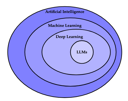
Machine Learning

One of the main sub-fields of artificial intelligence is machine learning, in which computer systems are developed to perform tasks without being explicitly programmed to do so by extrapolating from data. This is in contrast with other methods of artificial intelligence, such as rule-based expert systems, which encode facts and rules using formal, symbolic logic and perform logical deductions to draw conclusions.

Supervised Learning

Supervised learning is a type of machine learning which utilizes labeled data. The process of supervised learning proceeds roughly as follows:

• A model is selected to represent the task. A model is a specific function (in the mathematical sense) which maps inputs to outputs and is parameterized by parameters (numeric values) which control the mapping of inputs to outputs. The inputs and outputs numerically encode some data (e.g. text, pixels of an image) in an appropriate manner. Note that the term "model" is overloaded. It may refer to a specific parameterized function as we employ the term, or to the parameters themselves, or to a class of such functions, etc.
• A labeled training dataset is prepared somehow (either manually, or by extracting preexisting labeled data from some source) which consists of pairs of inputs and intended outputs called labels. The term supervisory signal is also used to refer to such labels.
• A so-called loss function is selected which quantifies the "loss'', i.e., the difference between the model's predicted output and the intended output.
• An optimization method is selected which is an algorithm for incrementally reducing the loss of the model.
• The model is trained by an iterative process consisting of inputting the inputs into the model to produce an output, computing the loss according to the input's respective label, and applying the optimization procedure to incrementally reduce the loss. The training process stops once some criterion is met.
• Once trained, the model may be applied to inputs that were not part of its training dataset. This is called generalization. Thus, the model is able to extrapolate from data.

Thus, the model "learns" the input-output mapping via the "training'' (optimization) process, and the labels "supervise'' the learning process by superintending the desired outcomes.

Self-Supervised Learning

In the process of self-supervised learning, supervisory signals (labels) are extracted from the data itself. For instance, many large language models are trained to predict which word will follow a given sequence of words. Their input is thus a sequence of words such as "Alice was beginning to get very'', and their output is the word predicted to come next, such as "tired''. Thus, the texts used to train such models already contain their own supervisory signals: given any sequence of words within the text, the supervisory signal is simply the next word in the text.

Deep Learning

Within machine learning, the sub-field of deep learning has become prevalent, in which a class of machine learning models called neural networks are employed to solve problems. In particular, LLMs are examples of deep learning models.

LLMs

One of the most prominent applications of deep learning is found in large language models (LLMs) such as the GPT (Generative Pre-trained Transformer) series of models produced by OpenAI, various versions of which underlie the popular ChatGPT application.

A large language model is a deep learning model trained on a comparatively large dataset and designed to generate text (often natural language text). The model is large in the sense that its training dataset consists of a comparatively large amount of text and in the sense that it contains a comparatively large number of parameters.

Remarkably, despite the impressive text generation capabilities of LLMs, they are trained to perform a comparatively straightforward task: to predict the next word following a given sequence of preceding words.

GPT

We will describe an architecture very similar to OpenAI's GPT-2 and GPT-3 architectures. The GPT 3.5 model was the basis for the original ChatGPT application. Although LLMs are rapidly evolving to incorporate new techniques, the core principles remain applicable, and thus it is worthwhile to understand these prototypical architectures.

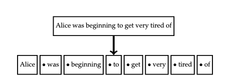
Tokenization

Tokenization is the process of decomposing a text into smaller individual units of text called tokens, as in the following figure.

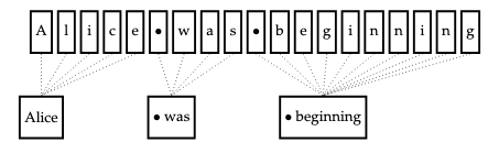
Alternatively, if text is conceived as a sequence of characters (symbols, such as letters, spaces, or punctuation), then tokenization can be construed as the process of grouping consecutive characters into tokens, as in the following figure. Computer systems represent text as sequences of characters.

Character Encoding

In computer systems, characters are represented using a character encoding. A character encoding assigns individual characters to unique numbers called code points. Each code point is represented according to an encoding scheme as a sequence of one or more bytes. The most common character encodings are ASCII (The American Standard Code for Information Interchange) and Unicode. For instance, both ASCII and Unicode assign the character "A'' to the code point \(65\) (in decimal). Since ASCII only defines a character set of 128 code points and each byte can encode up to \(2^8=256\) characters, its encoding scheme represents every code point using a single byte. However, Unicode defines several encoding schemes, the most common being UTF-8, which is a variable-length encoding (it encodes common characters using a single byte, but some characters may require multiple bytes).

Byte Pair Encoding

One of the most widely adopted tokenization algorithms is the byte pair encoding (BPE) algorithm. Our goal in this section is to indicate the gist of the algorithm, rather than all of its details (some of which vary among implementations).

With character-level BPE, the components of tokens are characters (or, equivalently, their code points). This can present problems, however:

• If characters are encountered during inference which were not encountered during training, the model will not know how to process such characters. However, the token vocabulary could be augmented with a special token UNK representing unknown characters.
• Alternatively, every character in the encoding scheme could be added to the vocabulary as an initialization step. However, Unicode contains a very large number of characters, so this would be inefficient.

With byte-level BPE, the components of tokens are bytes. Thus, the vocabulary could be initialized with one identifier for each unique byte value (of which there are only 256), etc. Then, since input is always a sequence of bytes and every byte is represented in the vocabulary, no matter what input is encountered during inference, it will always be able to be tokenized. We will describe byte-level BPE here.

The text is encoded in some standard encoding, typically UTF-8. The text is then treated as a sequence of bytes rather than a sequence of characters (due to the encoding scheme, certain characters may be represented as multiple bytes).

Often, there is an initialization phase which typically assigns each of the 256 byte values its own value as its identifier. Thus, the input can now be understood as a sequence of token identifiers rather than as a sequence of bytes. Then, the algorithm proceeds by identifying the most frequently occurring pairs of adjacent token identifiers in the input sequence. It then selects one, generates a new, hitherto unused, identifier to represent the pair, and replaces each occurrence of the pair in the input with this new token identifier. The algorithm proceeds iteratively until either a prescribed vocabulary size is achieved or there are no more pairs of adjacent token identifiers which occur more than once. Once the algorithm terminates, the vocabulary consists of all the generated token identifiers.

We will illustrate this in the following example (keep in mind that details may vary widely based on the implementation). Consider the following input text:

the cat sat on the mat.

Suppose that each character is encoded by a single byte and that this input corresponds to the following stream of bytes:

116 104 101 32 99 97 116 32 115 97 116 32 111 110 32 116 104 101 32 109 97 116 46

Suppose that we initialize our vocabulary inventory with one token identifier per byte (so, with values 0 through 255).

The most frequently occurring pair of bytes is 97 116 (corresponding to at). Suppose that we always select the pair with the first occurrence in the stream whenever there is a tie. We then generate a fresh identifier (say, 256) and replace each occurrence of the pair with this identifier.

116 104 101 32 99 256 32 115 256 32 111 110 32 116 104 101 32 109 256 46

We then map 116 104 (th) to 257

257 101 32 99 256 32 115 256 32 111 110 32 257 101 32 109 256 46

We then map 257 101 ([th]e) to 258.

258 32 99 256 32 115 256 32 111 110 32 258 32 109 256 46

We then map 258 32 ([the]<space>) to 259.

259 99 256 32 115 256 32 111 110 32 259 109 256 46

Finally, we map 256 32 ([at]<space>) to 260.

259 99 260 115 260 111 110 32 259 109 256 46

No more pairs of token identifiers remain in the input. The final vocabulary inventory is as follows:

• 0...255 map to themselves
• 256 \(\rightarrow\) 97 116 (at)
• 257 \(\rightarrow\) 116 104 (th)
• 258 \(\rightarrow\) 257 101 ([th]e)
• 259 \(\rightarrow\) 258 32 ([the]<space>)
• 260 \(\rightarrow\) 256 32 ([at]<space>)

BPE has the following advantages:

• There is no need for a special UNK token. Since inputs are treated as sequence of bytes and every byte is assigned a token identifier, it is not possible to encounter an unidentified token during inference.
• The size of the vocabulary is reduced (which is more efficient since much of the subsequent computation is proportional to the vocabulary size).
• Patterns in sub-word units can be discovered (e.g. suffixes such as -ed or -ing or prefixes such as un- in English).
• There is no need to define a vocabulary explicitly; it will be discovered from the corpus of texts. Additionally, this process works with multiple languages and with text which does not represent natural language (such as computer code, etc.).

Input Embeddings

The tokenization process associates tokens with numeric identifiers.

\[\text{Alice was beginning to get very tired} \rightarrow \texttt{43} ~\texttt{24} ~\texttt{97} ~\texttt{16} ~\texttt{20} ~\texttt{39} ~\texttt{86}.\]

The goal of a token embedding is to embed these token identifiers into a higher-dimensional vector space so that each token is represented by a vector of numbers rather than a single scalar number. The additional dimensions afford greater flexibility in the representation of tokens. Whereas the token identifiers are integer numbers, the components of their respective token embedding vectors are permitted to be non-integral, which also affords greater flexibility.

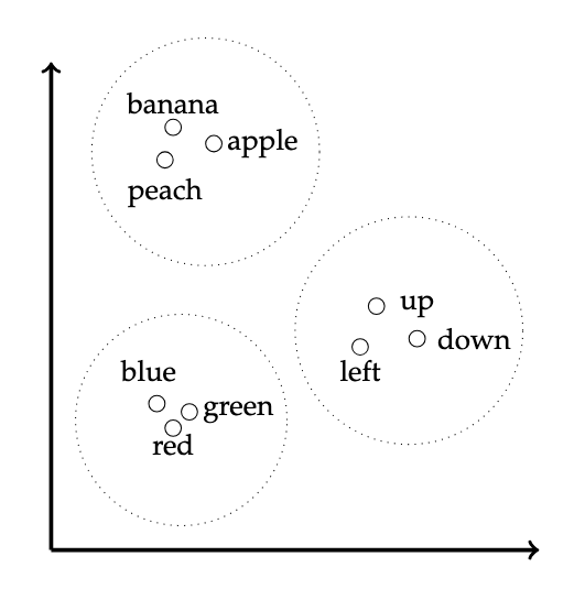
As a rough approximation, you could imagine that lexically related words will be grouped together and that multiple, independent groupings are permitted along different dimensions, as in the following figure. However, it is not necessary for the embedding process to proceed via groupings in this manner; this is just a rough illustration. The representation of tokens as vectors will be learned via the training process.

One simple, yet effective, method of embedding tokens is as follows: first, each token is associated with its respective one-hot encoding in which a token with identifier \(k\) is represented in an \(n\)-dimensional vector space (where \(n\) is the size of the token vocabulary) as an \(n\)-dimensional vector whose \((k+1)\)-th (assuming the identifiers start at \(0\) instead of \(1\)) component is \(1\) and whose other components are \(0\). Thus, for instance, if the vocabulary size is \(5\), the token with identifier \(2\) (i.e., the third token if the identifiers begin at \(0\)) would be represented as

\[\begin{bmatrix}0 \\ 0 \\ 1 \\ 0 \\ 0\end{bmatrix}.\]

The one-hot encoding of a token with identifier \(k\) can thus be defined as the map \(k \mapsto e_{k+1}\) (where \(e_{k+1}\) is the \((k+1)\)-th standard basis vector for \(\mathbb{R}^n\)).

An embedding is then a linear map between vector spaces, i.e., from the vocabulary space to the embedding space. If the vocabulary consists of \(n\) token identifiers and the selected embedding dimension is \(m\), then this is a linear map \(E : \mathbb{R}^n \rightarrow \mathbb{R}^m\). Every such linear map can be represented by an \(m \times n\) matrix of weights (which we will write as \(W\)), so that the embedding vector \(v\) is simply

\[v = We_{k+1}.\]

Writing \(W=(w_{ij})\) (where \(i\) is the row and \(j\) is the column), this is written

\[\begin{bmatrix}w_{11} & \dots & w_{1n} \\ \vdots & \ddots & \vdots \\ w_{m1} & \dots & w_{mn}\end{bmatrix} \begin{bmatrix}0 \\ \vdots \\ 1 \\ \vdots \\ 0\end{bmatrix} = \begin{bmatrix}w_{1k} \\ \vdots \\ w_{mk}\end{bmatrix}.\]

For example, if the vocabulary size is \(n=5\) and the embedding dimension is \(m=3\), then the embedding vector can be computed as follows:

\[\begin{bmatrix}0.1 & 0.4 & -0.3 & 0.9 & 0.6\\ 0.2 & -0.5 & 0.6 & 0.8 & 0.2\\ 0.4 & 0.2 & 0.7 & 0.8 & 1.2\\ \end{bmatrix} \begin{bmatrix}0 \\ 0 \\ 1 \\ 0 \\ 0\end{bmatrix} = \begin{bmatrix}-0.3 \\ -0.6 \\ 0.7\end{bmatrix}.\]

Since, \(We_{k+1} = e_{k+1}^TW\), we can also perform the same operation using the transpose of this matrix:

\[\begin{bmatrix}0 & 0 & 1 & 0 & 0\end{bmatrix} \begin{bmatrix}0.1 & 0.2 & 0.4\\ 0.4 & -0.5 & 0.2\\ -0.3 & 0.6 & 0.7\\ 0.9 & 0.8 & 0.8\\ 0.6 & 0.2 & 1.2 \end{bmatrix} = \begin{bmatrix}-0.3 & -0.6 & 0.7\end{bmatrix}.\]

Depending on how these matrices are represented, one may be more efficient than the other (for instance, if stored in row-major order, then the transpose representation will be more efficient). As you can see, the product of a matrix with a one-hot encoding merely selects a particular column (or row, depending on the representation) of the matrix. Thus, implementations of embeddings typically provide a specialized means for computing the embedding (e.g., by looking up the appropriate column or row directly) rather than actually performing the multiplication. However, for mathematical and conceptual purposes, a matrix multiplication is occurring.

Positional Embeddings

Word order is typically important in texts. However, neither the token embedding nor the self-attention mechanism (described subsequently) account for word order. A positional embedding embeds a token's position into the embedding vector space. The positional embedding can then be added to the token embedding to produce a final embedding. The position of a token can be relative or absolute. Here, we will use an absolute position embedding. The position will be the index of the token within the context window. The positional embedding then proceeds in the same manner as the token embedding, except that the one-hot representation of the position is used rather than the one-hot representation of the token identifier. Thus, the final embedding of a token with identifier \(k\) at position \(l\) (where positional indices start at \(0\)) is simply

\[W_te_{k+1} + W_pe_{l+1}\]

where \(W_t\) is the matrix of weights used for the token embedding and \(W_p\) is the matrix of weights used for the positional embedding.

Attention

Now, we will describe how to represent context as a vector. The notion of the context of a given token embedding (this word being the focus of the context) is formalized in terms of the sequence of words adjacent to this focus (including the focus itself).

Basic Attention

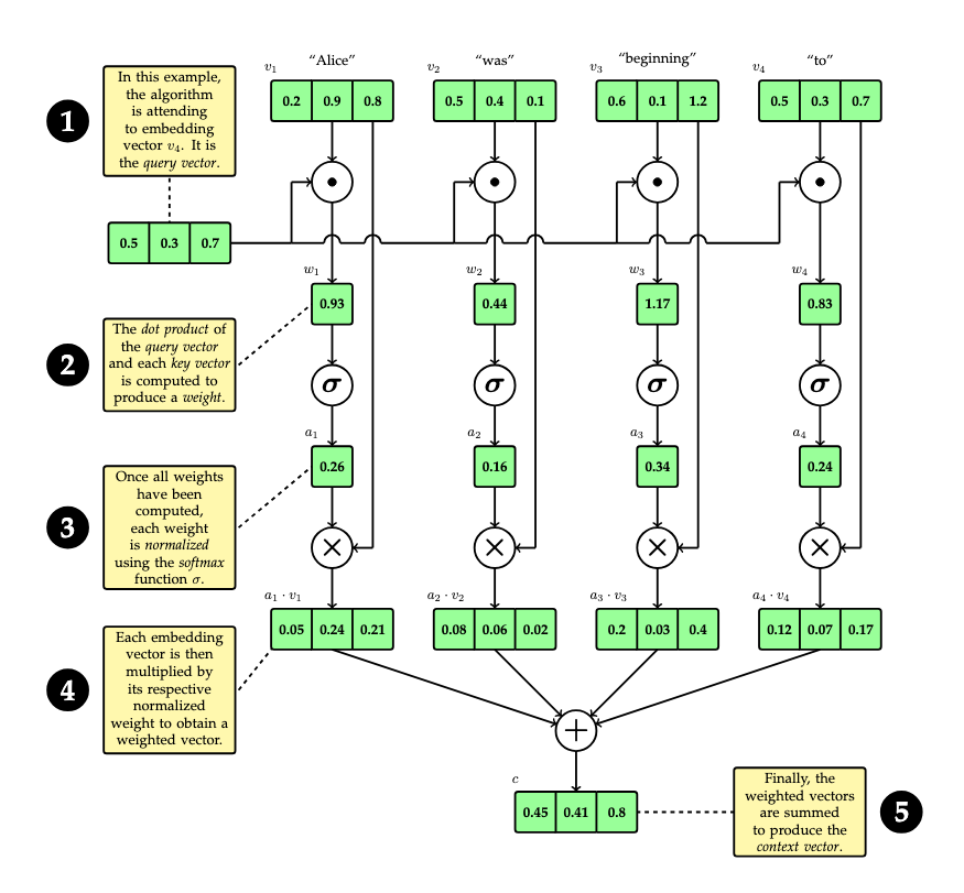
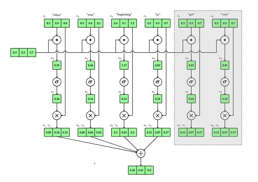
Suppose we define a context window of size 4 (i.e. consisting of 4 tokens). Such a small context window is unrealistic, and is chosen only for the purpose of illustration. Also, for the sake of simplicity, we will illustrate with words and punctuation, but remember that words and punctuation represent token embeddings, so that when we write "word" we really mean "token embedding", and that there is not a one-to-one relationship between words and token embeddings. Consider the following example (taken from the opening of Alice's Adventures in Wonderland):

Alice was beginning to get very tired of sitting by her sister on the bank, and of having nothing to do...

The bold, highlighted text indicates the current context window. Our goal is to represent the context of each word within the bounds of this window. We will attend to each word in the window, one at a time. Suppose that we are attending to the word "to" in this window. We refer to the word receiving attention as the query (database terminology has been co-opted). For each word in the context window (where each such word is called a key), we will compute a weight which somehow indicates the relevance of the key to the query. The dot product (inner product) of the respective embedding vectors is a good candidate for such a weight. Recall that the dot product \(a \cdot b\) of two vectors \(a,b \in \mathbb{R}^n\), where \(a = (a^1,\dots,a^n)\) and \(b =(b^i,\dots,b^n)\), is given by

\[a \cdot b = \sum_{i=1}^n a^i \cdot b^i.\]

Note that the dot product has the following geometric interpretation

\[a \cdot b = \lVert a \rVert \lVert b \rVert \cos \theta\]

where \(\theta\) is the angle between \(a\) and \(b\), as in the following figure.

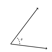
Thus, the dot product provides a measure of the "nearness" of two vectors. Thus, we can define the weight assigned to key vector \(k\) relative to query vector \(q\) as follows:

\[w(q, k) = q \cdot k.\]

Next, we want to normalize these weights such that they sum to \(1\) so that we can compute a context vector as a weighted sum of these vectors. We could simply average the weights as follows:

\[a(q, k) = \frac{w(q, k)}{\sum_{i=1}^n w(q,k)}.\]

However, the softmax function is often used because it promotes greater numerical stability during training. The softmax function \(\sigma\) is defined as follows for an \(n\)-dimensional vector \(v\):

\[\sigma(v) = (\sigma_1(v),\dots,\sigma_n(v))\]

where

\[\sigma_i(v) = \frac{e^{v^i}}{\sum_{j=1}^n e^{v^j}}.\]

The normalized attention weight (or attention score) of a key vector relative to a query vector is then defined as

\[a_i(q) = \sigma_i(w(q))\]

where

\[w(q) = (q \cdot v_1,\dots, q \cdot v_n).\]

Finally, the context vector assigned to query vector \(q\) is defined as the weighted sum of each of the key vectors in the context, using the respective attention score as the weight:

\[c(q) = \sum_{i=1}^n a_i(q) \cdot k_i.\]

Thus, for a window consisting of \(n\) tokens, \(n\) context vectors will be produced. In the example above, 4 context vectors would be computed. The following diagram indicates the basic attention mechanism for this example.

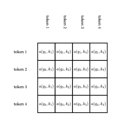
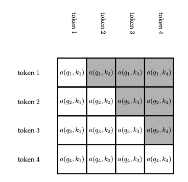
This scheme permits words which succeed a given word to be part of the word's context. We will amend this to only include words which precede a given word later. The following matrix indicates all of the attention scores with rows representing each query and columns representing each key.

The context window is a sliding window that is moved during training. The context window size and the stride (the positional increment between the starting index of one window and the starting index of the next window) are often configurable hyper-parameters of the training process. For instance, returning to our example, if the window size is 4 and the stride is 1, then the next window would be

Alice was beginning to get very tired of sitting by her sister on the bank, and of having nothing to do...

However, with a window size of 4 and a stride of 4, the next window would be

Alice was beginning to get very tired of sitting by her sister on the bank, and of having nothing to do...

There is typically a tradeoff between truncating potentially useful context and increasing training time.

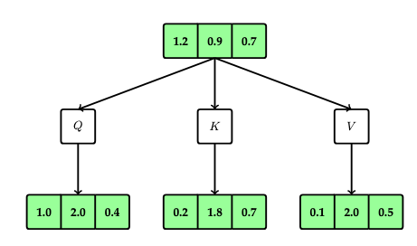
Parameterized Attention

Next, we will tease apart the various roles played by each embedding vector by parameterizing each by matrices:

• A matrix \(Q\) will determine the query vector for an embedding vector \(v\) as \(Qv\)
• A matrix \(K\) will determine the key vector for an embedding vector \(v\) as \(Kv\)
• A matrix \(V\) will determine the value vector for an embedding vector \(v\) as \(Vv\); the value vector is the vector against which the attention score is multiplied. Previously, the key vector was used for this role.

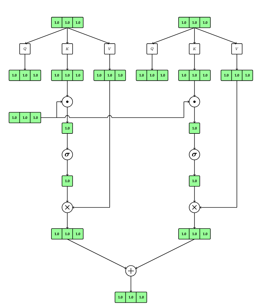
This is illustrated in the following diagram:

The process for computing a context vector is similar:

\[c(v) = \sum_{i=1}^n a_i(Qv) \cdot Vv_i\]

where

\[a_i(q) = \sigma_i(w(q))\]

and

\[w(q) = (q \cdot Kv_1,\dots, q \cdot Kv_n).\]

This is depicted in the following figure (but only for two vectors):

Causal Attention

Next, we will amend the attention mechanism such that it only considers key vectors which precede a given query vector. This ensures that causality is maintained (i.e., the words preceding a given word generally determine the word but the words succeeding this word generally do not determine the word). The term "causality" is related to temporal causality, i.e., past events determine present events but future events do not determine present events, etc.

The idea is very simple: simply ignore key vectors which succeed the query vector. This is illustrated in the following figure:

This can be accomplished in various manners. The following figure indicates the attention scores which are not considered for causal attention.

This can be accomplished in various ways. For instance, a mask can be applied, i.e., a matrix of values can be constructed and either multiplied or added (depending on the nature of the mask) to the computed scores in order to compute \(0\) for the irrelevant attention scores, such that, when the computation is performed, the irrelevant key vectors will essentially be excluded from the computation.

Thus, the calculation is amended as follows:

\[c(v_k) = \sum_{i=1}^k a_i(Qv_k) \cdot Vv_i\]

where

\[a_i(q) = \sigma_i(w(q))\]

and

\[w(q) = (q \cdot Kv_1,\dots, q \cdot Kv_n).\]

Multi-Head Attention

One final modification is called multi-head attention. In this variant, multiple independent context vectors are computed and then concatenated together to compute the final context vector. This is illustrated in the following figure.

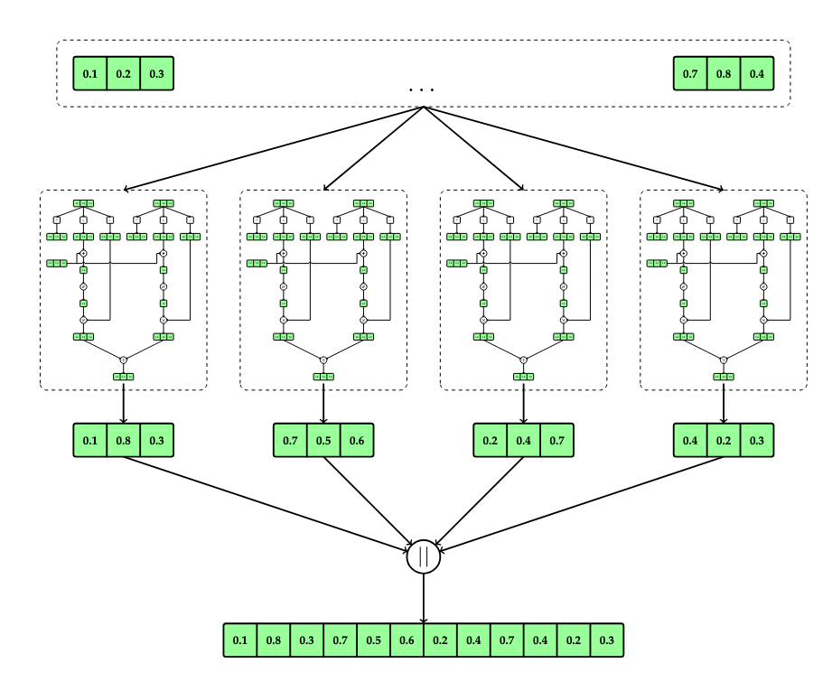
The final computation, where \(m\) is the number of independent context vectors, becomes

\[c(q) = c_1 \lVert \dots \lVert c_m\]

where \(\lVert\) denotes concatenation, i.e., \(a \lVert b = (a_1,\dots,a_n,b_1,\dots,b_n)\) and

\[c_i(v_k) = \sum_{j=1}^k a_{ij}(Q_iv_k) \cdot V_iv_j\]

where \(Q_i\), \(K_i\), and \(V_i\) are the matrices of weights corresponding to context vector \(c_i\) and

\[a_{ij}(q) = \sigma_j(w_i(q))\]

and

\[w_i(q) = (q \cdot K_iv_1,\dots, q \cdot K_iv_n).\]

Often, to promote greater numerical stability with floating-point numbers, the unnormalized attention weights are scaled by the inverse of the square root of the embedding dimension prior to normalization via softmax.

Neural Networks

Neural networks are composed of units called neurons, as depicted in the following figure. Each neuron accepts one or more inputs, which are multiplied by weights, one weight for each respective input. The products of the inputs and weights are summed. Optionally, a bias is added to this sum. Then, the sum is passed to an activation function, which is a non-linear function. The output of the activation function is the output of the neuron.

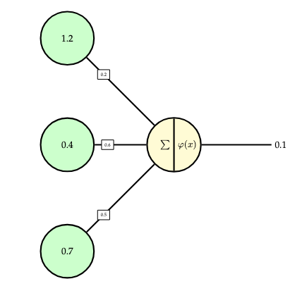
Thus, a neuron computes an output from an input as follows (where \(x = (x_1,\dots,x_n)\) are the inputs \(w=(w_1,\dots,w_n)\) are the weights, \(b\) is the bias, and \(\varphi\) is the activation function):

\[f(x) = \varphi\left(\left(\sum_{i=1}^n w_i \cdot x_i\right) + b\right).\]

This can be more succinctly expressed using the dot product (or, equivalently, matrix multiplication \(w^Tx\)):

\[f(x) = \varphi((w \cdot x) + b).\]

Activation Functions

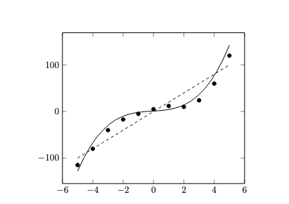
Activation functions introduce non-linearity, which permit neural networks to model more complex data. Without activation functions, neural networks would represent linear maps, and could not model non-linear relationships accurately (see the following figure).

There are many kinds of activation functions used in practice, but often rectifiers are used. The rectified linear unit (ReLU) function is defined as follows:

\[\mathrm{ReLU}(x) = \begin{cases} 0 & \text{if}~x < 0 \\ x & \text{otherwise}.\end{cases}\]

This can equivalently be defined as follows:

\[\mathrm{ReLU(x)} = \frac{x + \lvert x \rvert}{2}.\]

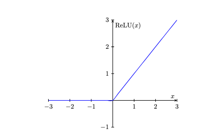
Thus, rectifiers map negative inputs to \(0\) and non-negative inputs to themselves.

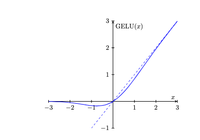
One serious technical problem with ReLU is that it is not a differentiable function, which makes it unsuitable for use with certain optimization techniques which require differentiable functions. Thus, certain differentiable approximations to ReLU are often used in practice. The GELU (Gaussian Error Linear Unit) function is one such example. It is defined as follows:

\[\mathrm{GELU}(x)=x \cdot \Phi(x),\]

where \(\Phi(x)\) is the cumulative distribution function (CDF) for the Gaussian distribution. Often, an approximation to this is used, which is defined as follows:

\[\mathrm{GELU}(x) \approx 0.5 \cdot x \cdot \left(1+ \tanh\left(\frac{2}{\pi} \cdot \left(x + 0.044715 \cdot x^3\right)\right)\right).\]

When considering the plot in the following figure, it becomes clear why this particular function is used: it asymptotically approximates the shape of the ReLU function.

Deep Learning

Neurons can be combined into networks, as depicted in the following figure. In such networks, inputs can propagate through multiple neurons and neurons can be chained together. Typically, neural networks are stratified into distinct layers (depicted by various colors in the figure). This stratification makes neural networks more manageable (since, as we will see, networks reduce to alternating series of matrix multiplications and activation function applications, that is, alternating series of linear and non-linear maps).

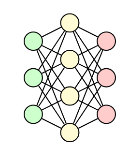
So-called deep neural networks are neural networks with many layers (at least 3 or more layers). The field of deep learning is concerned with the theory and application of deep neural networks to solve machine learning problems. Consider the following figure, which depicts a simple, three-layer neural network. This type of network is called a feedforward network since inputs are "fed forward" from one layer to the next (i.e., layers are not "skipped'' and there are no feedback "loops'', etc.).

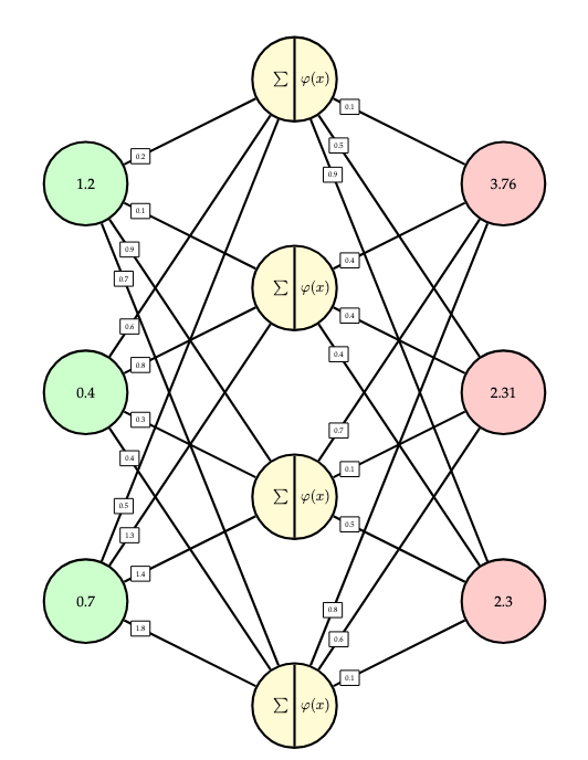
The concrete calculation performed by this particular network can be summarized as follows: first, the following matrix represents the weights of the first layer:

\[W_1 = \begin{bmatrix}0.2 & 0.6 & 0.5\\ 0.1 & 0.8 & 1.3\\ 0.9 & 0.4 & 1.4\\ 0.7 & 0.4 & 1.8\end{bmatrix}.\]

The summed inputs to the second layer are then computed as the product of this matrix with a vector of inputs:

\[\begin{bmatrix}0.2 & 0.6 & 0.5\\ 0.1 & 0.8 & 1.3\\ 0.9 & 0.4 & 1.4\\ 0.7 & 0.4 & 1.8\end{bmatrix}\begin{bmatrix}1.2 \\ 0.4 \\ 0.7\end{bmatrix} = \begin{bmatrix}0.83 \\ 1.35 \\ 2.18 \\ 2.26\end{bmatrix}.\]

Then, the GELU activation function is applied:

\[\mathrm{GELU\left(\begin{bmatrix}0.83 \\ 1.35 \\ 2.18 \\ 2.26\end{bmatrix}\right)} = \begin{bmatrix}0.62 \\ 1.17 \\ 2.11 \\ 2.2\end{bmatrix}.\]

Finally, the weights of the second layer are represented as

\[W_2 = \begin{bmatrix}0.1 & 0.4 & 0.7 & 0.8 \\ 0.5 & 0.4 & 0.1 & 0.6 \\ 0.9 & 0.4 & 0.5 & 0.1\end{bmatrix}\]

and this matrix is multiplied by the outputs of the previous layer to obtain

\[\begin{bmatrix}0.1 & 0.4 & 0.7 & 0.8 \\ 0.5 & 0.4 & 0.1 & 0.6 \\ 0.9 & 0.4 & 0.5 & 0.1\end{bmatrix}\begin{bmatrix}0.62 \\ 1.17 \\ 2.11 \\ 2.2\end{bmatrix} = \begin{bmatrix}3.76 \\ 2.31 \\ 2.3\end{bmatrix}.\]

Thus, the entire calculation is

\[W_2 \cdot \varphi(W_1 \cdot x).\]

Thus, such feedforward networks are just alternations of linear maps (matrix multiplication) and non-linear maps (activation functions). Matrix multiplication is efficient to compute as well since there are many independent operations (scalar additions and multiplications) which can be performed in parallel (e.g., using a graphics processing unit).

Transformers

Next, we will describe the transformer architecture, a particular neural network architecture which is used within many large language models. Neural networks are often modular in design, that is, they consists of multiple smaller sub-networks. We will describe various blocks (i.e. sub-networks) which comprise components of the transformer architectures.

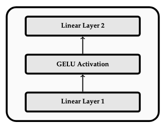
Feedforward Block

The feedforward block is one of the most basic components, and consists of a simple feedforward neural network consisting of a linear layer, a GELU activation layer, and a second linear layer (essentially the same as the feedforward network described above). This is depicted in the following figure:

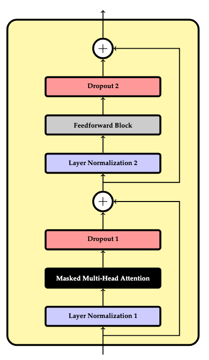
Transformer Block

The transformer block is the primary component of the transformer architecture. It consists of the following parts:

1. A normalization layer which normalizes its inputs such that they enjoy desirable statistical properties (i.e., a mean of \(0\) and a standard deviation of \(1\)). This promotes greater numerical stability with the use of floating-point arithmetic.
2. An instance of the masked multi-head attention mechanism.
3. A dropout layer which applies a randomized mask to "drop" (i.e. zero) particular weight parameters as a heuristic to prevent over-reliance on any particular parameters.
4. A shortcut connection which combats the vanishing gradient problem by adding the original input to the output of the prior 3 layers.
5. A second normalization layer.
6. A feedforward block.
7. A second dropout layer.
8. A final shortcut connection which combines the output from the prior shortcut to the final output.

This is depicted in the following figure:

The Architecture

We can now describe the overall transformer architecture. It consists of the following sequence of components:

1. A token embedding layer.
2. A positional embedding layer.
3. An initial dropout layer.
4. \(N\) instances of the transformer block in a chain.
5. A final normalization layer.
6. A vocabulary embedding layer which converts the output (which is a sequence of context vectors) to a sequence of discrete probability distributions over the vocabulary. These distributions can be sampled in order to select the next token. This will be explained subsequently in the section on output embeddings.

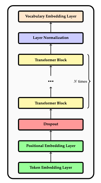
Thus, the transformer accepts a sequence of tokens (within a context window) as input, and produces a sequence of probability distributions as outputs (one per token in the context window), where each distribution can be sampled to determine the output token. This information is useful for training, but only the ultimate such distribution is used during inference, since it represents the distribution of tokens which succeed the entire input sequence. This is depicted in the following figure.

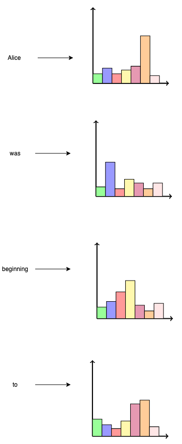
The ultimate distribution can then be sampled according to an appropriate sampling strategy in order to determine the next token:

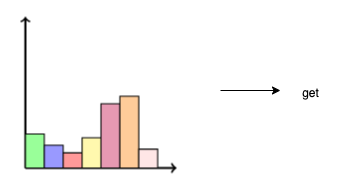
Thus, in this manner, the next token can be determined:

\[\text{Alice was beginning to} \rightarrow \text{get}.\]

Output Embeddings

The transformer architecture transforms a sequence of token identifiers to a sequence of context vectors. We then want to embed each context vector in the vector space \(\mathbb{R}^m\), where \(m\) is the vocabulary size (the number of distinct token identifiers in the vocabulary inventory produced during the tokenization training process). Thus, there will be one component of the embedded vector per token in the vocabulary. This embedding, like all embeddings, is a linear map with signature \(\mathbb{R}^n \rightarrow \mathbb{R}^m\), where \(n\) is the dimension of the context vectors. Since each such linear map is representable by a matrix, this is accomplished via a trainable matrix of weights.

The output of this embedding process is then normalized using the softmax function such that each component of the resultant normalized vector represents the probability that the token identifier, represented by the index of the component within the vector, is the token which succeeds the respective context. This is depicted in the following figure.

Then, a sampling strategy can be used to select a token identifier from this distribution. The most obvious strategy is to select the most likely token, i.e. the token with the highest probability:

\[\mathrm{argmax}(p(x)).\]

However, more interesting and varied text can be produced by using alternative sampling strategies (e.g. selecting among the top \(k\) results).

This process can be understood as computing the conditional probability of a token given a sequence of preceding tokens.

Training

Next, we will describe the process of training a large language model, i.e., the process of determining the values of its various parameters (which essentially amount to the values of all the various matrices used throughout).

Cross-Entropy

The usual loss function used when training LLMs is cross-entropy. Cross-entropy is an information-theoretic measure. The cross-entropy between two probability distributions \(p\) and \(q\) measures the average number of bits (in the information-theoretic sense) required to identify an event drawn from the common support \(\mathcal{X}\) (set of events) of these distributions when the coding scheme employed is the estimated distribution \(q\) rather than the true distribution \(p\). It thus provides a measure of the difference between the two distributions, i.e., the failure of the estimated distribution to conform to the true distribution. It is defined for discrete distributions \(p\) and \(q\) as follows:

\[H(p, q) = -\sum_{x \in \mathcal{X}} p(x) \cdot \log_2(q(x)).\]

In the context of LLMs, we are performing a classification of a sequence of tokens where the class label is the token which succeeds the sequence within the training corpus. The "events" are the token identifiers. Thus, there is one distribution \(p\) per sequence of tokens. The distribution \(q\) is the estimated distribution output from the model. The true distribution \(p\) is unknown, so a "one-hot" distribution with \(p(x_i) = 1\) where \(x_i\) is the supervisory label for the \(i\)-th sample in the dataset and \(p(x) = 0\) otherwise is used. The cross-entropy then simplifies to

\[-\log_2(q(x_i)).\]

The average over the dataset is then used as the loss function (where \(T\) refers to the dataset):

\[H(T, q) = -\sum_{i=1}^n \log_2(q(x_i)).\]

When batching is used, this will be computed over each batch instead of the entire dataset.

Derivatives

In this section, we will review basic differential calculus. Refer to the following posts for more information about derivatives:

• Derivatives on Normed Vector Spaces
• Total Derivatives
• Differentials

The goal of the optimization process is to incrementally adjust the parameters of the neural network such that the value of the loss function decreases. Thus, we require a method for measuring how incremental changes in the inputs of functions affect the outputs of functions. Directional derivatives provide such a mechanism.

Directional Derivatives

Consider a function \(f : \mathbb{R}^n \rightarrow \mathbb{R}^m\). To evaluate the change in the input of \(f\), we fix a point \(p \in \mathbb{R}^n\) in the domain of \(f\) and consider how the output of \(f\) changes as the input of \(f\) deviates from \(p\) for a particular amount \(t \in \mathbb{R}\) in a fixed direction \(v \in \mathbb{R}^n\). The path of deviation from \(p\) can be parameterized as \(p + t \cdot v\). The parameter \(t\) therefore provides a measure of the change in the input. The change \(\Delta^t_pf(v) \in \mathbb{R}^m\) in the output of \(f\) is defined as follows:

\[\Delta^t_pf(v) = f(p + t \cdot v) - f(p).\]

We will express the relationship between the output and input as a ratio of the change in the output to the change in the input:

\[\frac{\Delta \text{Output}}{\Delta \text{Input}}.\]

Note that, while \(t\) is a scalar value, \(\Delta^t_pf(v) \in \mathbb{R}^m\) is, in general, a vector value (unless \(m=1\)):

\[\frac{\Delta \text{Output}}{\Delta \text{Input}} = \frac{\left(\Delta \text{Output}_1,\dots,\Delta \text{Output}_m\right)}{\Delta \text{Input}}.\]

Thus, there are effectively \(m\) ratios, one per dimension. In particular, according to our definitions above:

\[\frac{\Delta \text{Output}}{\Delta \text{Input}} = \frac{\Delta^t_pf(v)}{t} = \frac{f(p+t\cdot v)}{t}.\]

We cannot actually measure this ratio at the point \(p\), i.e., when \(t=0\), since its value would be \(\vec{0}/0\), which is undefined. Instead, we want to measure an appropriate value for arbitrarily small values of \(t\) in order to understand the input-output relationship in an arbitrarily small vicinity of the point \(p\). Thus, we want to compute the limit of this ratio as \(t\) approaches \(0\), namely

\[D_pf(v) = \lim_{t \to 0}\frac{f(p+t \cdot v - f(p))}{t}.\]

By definition, if such a limit exists, it is the (demonstrably unique) vector \(L \in \mathbb{R}^m\) such that, for any "error" threshold \(\varepsilon > 0\), there exists a \(\delta > 0\) such that, whenever \(\lvert t \rvert < \delta\), it follows that

\[\left \lVert \frac{f(p + t \cdot v) - f(p)}{t} - L \right \rVert < \varepsilon.\]

In other words, for any "error" threshold whatsoever, we can find a value of the parameter \(t\) such that the magnitude of the difference between the value of the ratio at \(t\) and the limit \(L\) is below this threshold, i.e., the ratio gets as close to the limit as we require.

If such a limit \(D_pf(v)\) exists, it is called the directional derivative of \(f\) at the point \(p\) in the direction \(v\).

Partial Derivatives

Partial derivatives are an important special case of directional derivatives. A partial derivative is a directional derivative in the direction of one of the standard basis vectors \(e_1,\dots,e_n\) for \(\mathbb{R}^n\) (i.e., in the direction of one of the "coordinate axes", if we think geometrically about vectors). Recall that the standard basis vectors are defined as follows:

\[e_1 = (1,0,\dots,0), e_2 = (0,1,\dots,0),\dots,e_n = (0,0,\dots,1).\]

The partial derivative of a function \(f : \mathbb{R}^n \rightarrow \mathbb{R}^m\) at a point \(p \in \mathbb{R}^n\) with respect to its \(i\)-th parameter \(x^i\) is written as \((\partial f/\partial x^i)(p)\) and defined as follows:

\[\frac{\partial f}{\partial x^i}(p) = D_pf(e_i) = \lim_{t \to 0}\frac{f(p + t \cdot e_i) - f(p)}{t}.\]

Total Derivatives

The difference function \(\Delta_pf\) measures the change in the output of a function \(f : \mathbb{R}^n \rightarrow \mathbb{R}^m\) as its input deviates from a point \(p \in \mathbb{R}^n\) in a particular direction \(v \in \mathbb{R}^n\) (and is thus a non-parametric version of \(\Delta^t_pf\) defined previously):

\[\Delta_pf(v) = f(p + v) - f(p).\]

The total derivative \(df_p : \mathbb{R}^n \rightarrow \mathbb{R}^m\) of \(f\) at the point \(p\) (also called the differential of \(f\) at the point \(p\)) is the best linear approximation of the difference function, meaning that, \(df_p\) is a linear map, and, for every \(v \in \mathbb{R}^n\),

\[\Delta_pf(v) = df_p(v) + o\left(\lVert v \rVert\right),\]

which is a special notation which means that

\[o\left(\lVert v \rVert\right) = \Delta_pf(v) - df_p(v),\]

i.e., \(o\) is a term which exactly represents the error in the approximation, and, furthermore

\[\lim_{v \to 0} \frac{\lVert \Delta_pf(v) - df_p(v) \rVert}{\lVert v \rVert}.\]

In other words, \(\lVert \Delta_pf(v) - df_p(v) \rVert\), the magnitude of the discrepancy between the difference function and the differential \(df_p\), vanishes "faster" than \(\lVert v \rVert\), the magnitude of \(v\), vanishes.

If the total derivative \(df_p\) exists at a point \(p\), then \(f\) is said to be differentiable at \(p\), and, if \(f\) is differentiable at all points in its domain, then \(f\) is simply said to be differentiable.

It is possible to demonstrate that, if a function \(f : \mathbb{R}^n \rightarrow \mathbb{R}^m\) is differentiable at a point \(p\), then its value at each vector \(v\) is equal to the respective directional derivative at \(p\) in the direction \(v\):

\[df_p(v) = D_pf(v).\]

Thus, the differential is a linear map which sends each vector \(v\) in the domain to its respective directional derivative.

The Jacobian Matrix

Every linear map can be represented (with respect to bases for its domain and codomain) as a matrix. In particular, every linear map \(A : \mathbb{R}^n \rightarrow \mathbb{R}^m\) can be represented (with respect to the standard bases \((e_1,\dots,e_n)\) for \(\mathbb{R}^n\) and \((e_1,\dots,e_m)\) for \(\mathbb{R}^m\)) as a matrix. This is accomplished by a twofold decomposition.

First, the input of \(A\) is decomposed in the domain of \(A\) in terms of the standard basis for \(\mathbb{R}^n\) as follows:

\begin{align}A(x) &= A(x^1 \cdot e_1 + \dots + x^n \cdot e_n) \\&= x^1 \cdot A(e_1) + \dots + x^n \cdot A(e_n).\end{align}

Second, the output of \(A\) is decomposed in the codomain of \(A\) in terms of the component functions \(A^i\) with respect to the standard basis for \(\mathbb{R}^m\) as follows:

\begin{align}A(x) &= A^1(x) \cdot e_1 + \dots + A^m(x) \cdot e_m \\&= \begin{bmatrix}A^1(x) \\ \vdots \\ A^m(x)\end{bmatrix}.\end{align}

Putting each of these two decompositions together yields

\begin{align}A(x) &= x^1 \cdot A(e_1) + \dots + x^n \cdot A(e_n) \\&= x^1 \cdot \begin{bmatrix}A^1(e_1) \\ \vdots \\ A^m(e_1)\end{bmatrix} + \dots + x^n \cdot \begin{bmatrix}A^1(e_n) \\ \vdots \\ A^m(e_n)\end{bmatrix} \\&= \begin{bmatrix}A^1(e_1) & \dots & A^1(e_n) \\ \vdots & \ddots & \vdots \\ A^m(e_1) & \dots & A^m(e_n)\end{bmatrix}\cdot \begin{bmatrix}x^1 \\ \vdots \\x^n\end{bmatrix}.\end{align}

Thus, the matrix

\[\begin{bmatrix}A^1(e_1) & \dots & A^1(e_n) \\ \vdots & \ddots & \vdots \\ A^m(e_1) & \dots & A^m(e_n)\end{bmatrix}\]

represents the linear map \(A\) in terms of the standard bases.

Limits in \(\mathbb{R}^m\) are computed component-wise, which means that

\[\lim_{h \to a}f(h) = \left(\lim_{h \to a}f^1(h),\dots,\lim_{h \to a}f^m(h)\right).\]

In particular, it follows that

\[df_p(v) = \left(df^1_p(v),\dots,df^m_p(v)\right).\]

Since differentials are linear maps, they also can be represented in terms of matrices as follows:

\begin{align}df_p(v) &= v^1 \cdot df_p(e_1) + \dots + v^n \cdot df_p(e_n) \\&= v^1 \cdot \begin{bmatrix}df^1_p(e_1) \\ \vdots \\ df^m_p(e_1)\end{bmatrix} + \dots + v^n \cdot \begin{bmatrix}df^1_p(e_n) \\ \vdots \\ df^m_p(e_n)\end{bmatrix} \\&= \begin{bmatrix}df^1_p(e_1) & \dots & df^1_p(e_n) \\ \vdots & \ddots & \vdots \\ df^m_p(e_1) & \dots & df^m_p(e_n)\end{bmatrix}\cdot \begin{bmatrix}v^1 \\ \vdots \\v^n\end{bmatrix} \\&= \begin{bmatrix}D_pf^1(e_1) & \dots & D_pf^1(e_n) \\ \vdots & \ddots & \vdots \\ D_pf^m(e_1) & \dots & D_pf^m(e_n)\end{bmatrix}\cdot \begin{bmatrix}v^1 \\ \vdots \\v^n\end{bmatrix} \\&= \begin{bmatrix}\frac{\partial f^1}{\partial x^1}(p) & \dots & \frac{\partial f^1}{\partial x^n}(p) \\ \vdots & \ddots & \vdots \\ \frac{\partial f^m}{\partial x^1}(p) & \dots & \frac{\partial f^m}{\partial x^n}(p)\end{bmatrix}\cdot \begin{bmatrix}v^1 \\ \vdots \\v^n\end{bmatrix}.\end{align}

This \(m\times n\) matrix of partial derivatives of component functions is called the Jacobian matrix:

\[J_pf = \begin{bmatrix}\frac{\partial f^1}{\partial x^1}(p) & \dots & \frac{\partial f^1}{\partial x^n}(p) \\ \vdots & \ddots & \vdots \\ \frac{\partial f^m}{\partial x^1}(p) & \dots & \frac{\partial f^m}{\partial x^n}(p)\end{bmatrix}.\]

Thus, every total derivative is represented by its respective Jacobian matrix in the sense that

\[df_p(v) = (J_pf) v.\]

The Chain Rule

One can prove various theorems which establish rules which enable the calculation of derivatives. One of the most important rules is the chain rule which permits the decomposition of arbitrarily complex expressions into smaller expressions. The chain rule for total derivatives states that, for any functions \(f : \mathbb{R}^n \rightarrow \mathbb{R}^m\) and \(g : \mathbb{R}^m \rightarrow \mathbb{R}^l\), the total derivative \(d(g \circ f)_p\) of the composite function \(g \circ f\) at a point \(p\) is given by the following expression:

\[d(g \circ f)_p = dg_f(p) \circ df_p.\]

Since the total derivative is a linear map and is represented by its respective Jacobian matrix, and since the composition of linear maps is represented by the product of the respective matrices representing the individual linear maps, it follows that the chain rule for total derivatives can be expressed as follows:

\begin{align}J_p(g\circ f) &= (J_{f(p)}g)(J_pf) \\&= \begin{bmatrix}\frac{\partial g^1}{\partial y^1}(f(p)) & \dots & \frac{\partial g^1}{\partial y^m}(f(p)) \\ \vdots & \ddots & \vdots \\ \frac{\partial g^l}{\partial y^1} (f(p)) & \dots & \frac{\partial g^l}{\partial y^m}(f(p))\end{bmatrix} \begin{bmatrix}\frac{\partial f^1}{\partial x^1}(p) & \dots & \frac{\partial f^1}{\partial x^n}(p) \\ \vdots & \ddots & \vdots \\ \frac{\partial f^m}{\partial x^1} (p)& \dots & \frac{\partial f^m}{\partial x^n}(p)\end{bmatrix}.\end{align}

Gradients

In the special case of a function \(f : \mathbb{R}^n \rightarrow \mathbb{R}\), if there exists a matrix which represents the directional derivative \(D_pf\), which, in this case, would be a \(1 \times n\) matrix, or, equivalently, a row vector \((\nabla f(p))^T\) with corresponding column vector \(\nabla f(p)\), then this means that

\[D_pf(v) = (\nabla f(p))^Tv = \nabla f(p) \cdot v.\]

If there exists one such \(\nabla f(p)\) for every point \(p\), i.e., there exists a vector field \(\nabla f : \mathbb{R}^n \rightarrow \mathbb{R}^n\) such that \(D_pf(v) = \nabla f(p) \cdot v\) for every point \(p\), then \(\nabla f\) is called the gradient of \(f\).

If \(f\) is differentiable at \(p\), then it is represented by its Jacobian matrix, which will be a \(1 \times n\) matrix, or, equivalently a row vector, so that

\[df_p(v) = (J_pf)v = \begin{bmatrix}\frac{\partial f}{\partial x^1}(p) & \dots & \frac{\partial f}{\partial x^n}(p)\end{bmatrix} \begin{bmatrix}v^1 \\ \vdots \\ v^n\end{bmatrix}.\]

Then, since \(df_p(v) = D_pf(v) = (J_pf)v\), it follows that

\[D_pf(v) = \begin{bmatrix}\frac{\partial f}{\partial x^1}(p) & \dots & \frac{\partial f}{\partial x^n}(p)\end{bmatrix} \begin{bmatrix}v^1 \\ \vdots \\ x^n\end{bmatrix} = \begin{bmatrix}\frac{\partial f}{\partial x^1}(p) \\ \vdots \\ \frac{\partial f}{\partial x^n}(p)\end{bmatrix} \cdot \begin{bmatrix}v^1 \\ \vdots \\ v^n\end{bmatrix},\]

and hence

\[\nabla f(p) = \begin{bmatrix}\frac{\partial f}{\partial x^1}(p) \\ \vdots \\ \frac{\partial f}{\partial x^n}(p)\end{bmatrix}.\]

The gradient evaluated at a point \(p\) indicates the direction of steepest ascent. For an intuitive explanation, consider the fact that the dot product \(\nabla f(p) \cdot v\) will attain its greatest value when \(\nabla f(p)\) and \(v\) are parallel. Thus, the gradient is useful for optimization since it indicates which direction to proceed in order to move toward a local maximum of the function. Conversely, the negation of the gradient indicates which direction to proceed in order to move toward a local minimum of the function.

Gradient Descent

The goal when training a neural network is to minimize the loss of the network with respect to a given loss function which quantifies the loss. The neural network can be modeled as a function \(f : \mathbb{R}^n \rightarrow \mathbb{R}^m\) and the loss function can be modeled as a function \(L : \mathbb{R}^m \rightarrow \mathbb{R}\). Thus, the goal of training is to minimize the value of the composite function \(F : \mathbb{R}^n \rightarrow \mathbb{R} = L \circ f\).

The gradient \(\nabla f(p)\) indicates the direction of greatest ascent relative to a point \(p\). Thus, the direction of greatest descent is \(-\nabla f(p)\). Since the gradient is the transpose of the derivative, its norm likewise indicates the magnitude of this ascent. We are primarily concerned with the relative magnitude rather than the absolute magnitude (i.e., the magnitude of ascent at a given point relative to the magnitude of ascent at other points). Thus, for any scalar factor \(\eta\), \(-\eta \cdot \nabla f(p)\) will still point in the direction of greatest decrease, at will preserve proportionality of the relative magnitudes of decrease at various points \(p\). This, suggests a systematic procedure for searching for a local minimum of a function:

1. Choose a starting point \(p_0\) (perhaps randomly). Set \(i=0\).
2. Compute \(\nabla f(p_i)\).
3. Compute the next point \(p_{i+1} = p_i - \eta \cdot \nabla f(p)\).
4. Proceed to step 2 with \(i \leftarrow i+1\).

This procedure continues indefinitely until some criterion is met. In the context of machine learning, the factor \(\eta\) is called the learning rate. If the learning rate is too great, the optimization procedure may continually "overshoot" the local minimum and may diverge. However, if the learning rate is too small, the optimization procedure may converge too slowly.

Note that the "direction of greatest descent" is relative to a given point \(p\), and thus only indicates a local minimum. If you visualize the graph of a function as a collection of hills and valleys, then a local minimum is simply the nearest "valley".

LLMs will typically work with non-convex "objective" functions with multiple local minima, so finding a global minimum is not guaranteed, but often local minima suffice in practice.

In the context of supervised learning, there is an entire collection of loss functions \(L_i\), one per sample in the training dataset. The usual goal is to minimize the average loss so that the loss function \(L\) is defined as

\[L(p) = \sum_{i=1}^n L_i(p).\]

Gradient descent then amounts to computing

\[\nabla L(p) = \sum_{i=1}^n \nabla L_i(p).\]

Thus, an entire collection of gradient values \(\nabla L_i(p)\) at the point \(p\) must be evaluated. This can be quite costly for many training datasets, which might be very large. Instead, a variant of gradient descent called stochastic gradient descent is often used in which a randomly selected subset of \(k\) items of the training dataset is used (where \(k < n\)). The gradient is then approximated as

\[\nabla L(p) \approx \sum_{i=1}^k \nabla L_i(p).\]

Backpropagation

We require an algorithm for systematically computing the gradients required for stochastic gradient descent in an efficient manner. The primary algorithm for doing so is called backpropagation. Backpropagation is perhaps best understood through examples, so we will consider several examples.

Example

Consider the following simple neural network (where the activation function \(\varphi\) is defined as \(\varphi = \sin\)) and the loss function \(\varepsilon\) is defined as \(\varepsilon(z) = (z-\bar{z}_i)^2\), where \(\bar{z}_i\) is the supervisory label associated with input \(i\):

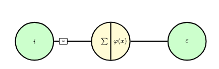
We will depict this network as a computational graph, which is a directed acyclic graph which represents an expression and explicitly indicates the mathematical operations within the network. The following computational graph represents the simple neural network above:

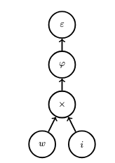
Next, we will represent this graph as the composition of several functions, one function per level of the graph. This graph represents the function \(F : \mathbb{R}^2 \rightarrow \mathbb{R}\) defined as

\[F(w,i) = (\sin(w \cdot i) - \bar{z}_i)^2.\]

We are only interested in optimizing this function with respect to the weight parameter \(w\), so we fix an input \(i\) and a supervisory label \(\bar{z}_i\) and define a function \(\bar{F} : \mathbb{R} \rightarrow \mathbb{R}\) as follows:

\[\bar{F}(w) = F(w, i).\]

We then define \(\bar{F}\) as the composite

\[\bar{F} = h \circ g \circ f\]

where

• \(f(w) = w \cdot i\),
• \(g(y) = \varphi(y) = \sin(y)\),
• \(h(z) = \varepsilon(z) = (z-\bar{z}_i)^2\).

To compute the gradient \(\nabla \bar{F}(p)\) at a point \(p=w\), we can apply the chain rule. The respective Jacobian matrices are as follows:

• \(J_pf = \begin{bmatrix}\frac{\partial f}{\partial w}(p)\end{bmatrix}\),
• \(J_{f(p)}g = \begin{bmatrix}\frac{dg}{dy}(f(p))\end{bmatrix}\),
• \(J_{g(f(p))}h = \begin{bmatrix}\frac{dh}{dz}(g(f(p)) \end{bmatrix}\).

Thus, the composite \(\bar{F}\) is represented as follows:

\[J_p\bar{F} = J_p(h \circ g \circ f) = \begin{bmatrix}\frac{dh}{dz}(g(f(p)) \end{bmatrix}\begin{bmatrix}\frac{dg}{dy}(f(p))\end{bmatrix}\begin{bmatrix}\frac{\partial f}{\partial w}(p)\end{bmatrix}.\]

Thus, the final gradient is the scalar value

\[\nabla \bar{F}(p) = \frac{dh}{dz}(g(f(p)) \frac{dg}{dy}(f(p))\frac{\partial f}{\partial w}(p).\]

We compute each of these partial derivatives as follows:

• \(\frac{df}{di}(p) = w\),
• \(\frac{dg}{dy}(f(p)) = \cos(f(p)) = \cos(w \cdot i)\),
• \(\frac{dh}{dz}(g(f(p)) = 2 \cdot (g(f(p)) - \bar{z}) = 2 \cdot (\sin(w \cdot i) - \bar{z}_i)\).

If \(w = 0.1\), \(i = 1.1\), \(\bar{z}_i = 0.8\), then we compute

\begin{align}i \cdot \cos(w \cdot i) \cdot 2 \cdot (\sin(w \cdot i) - \bar{z}_i) &= 1.1 \cdot \cos(0.1 \cdot 1.1) \cdot 2 \cdot (\sin(0.1 \cdot 1.1) - 0.8) \\&\approx -1.51.\end{align}

Next, consider the following crucial observations:

• There is one backward path from a sink node (labeled \(\varepsilon\)) to a source node (labeled \(w\)) representing a weight.
• The product \(\frac{dh}{dz}(g(f(p)) \frac{dg}{dy}(f(p))\frac{\partial f}{\partial w}(p)\) corresponds to this path.
• Each term of this product represents an intermediate node (an operation node) within the graph, e.g., \(\frac{dg}{dy}(f(p))\) represents the node labeled \(\varphi=\sin\).

Example

Consider another example of backpropagation with respect to the following simple neural network:

The computational graph corresponding to this network is depicted in the following figure:

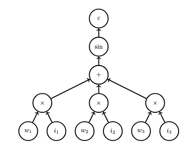
This graph represents the function \(F : \mathbb{R}^6 \rightarrow \mathbb{R}\) defined as follows (where \(\bar{v}_i\) is the supervisory label corresponding to input \(i = (i_1,i_2,i_3)\)):

\[F(w_1,w_2,w_3,i_1,i_2,i_3) = (\sin(w_1 \cdot i_1 + w_2 \cdot i_2 + w_3 \cdot i_3) - \bar{v}_i).\]

Again, we fix a particular input \(i = (i_1,i_2,i_3)\) and define

\[\bar{F}(w_1,w_2,w_3) = F(w_1,w_2,w_3,i_1,i_2,i_3).\]

This function is a composite of several functions (one per level of the graph), defined as

\[\bar{F} = \varepsilon \circ h \circ g \circ f\]

where

• \(f(w_1,w_2,w_3) = (w_1 \cdot i_1, w_2 \cdot i_2, w_3 \cdot i_3\),
• \(g(y_1,y_2,y_3) = y_1 + y_2 + y_3\),
• \(h(z) = \sin(z)\),
• \(\varepsilon(v) = (v - \bar{v}_i)^2\).

The Jacobian matrices are as follows (where \(p=(w_1,w_2,w_3)\)):

• \(J_pf =\begin{bmatrix}
  \frac{\partial f^1}{\partial w_1}(p) & \frac{\partial f^1}{\partial w_2}(p) & \frac{\partial f^1}{\partial w_3}(p) \\ \frac{\partial f^2}{\partial w_1}(p) & \frac{\partial f^2}{\partial w_2}(p) & \frac{\partial f^2}{\partial w_3}(p) \\
  \frac{\partial f^3}{\partial w_1}(p) & \frac{\partial f^3}{\partial w_2}(p) & \frac{\partial f^3}{\partial w_3}(p)
  \end{bmatrix}\),
• \(J_{f(p)}g = \begin{bmatrix}\frac{\partial g}{\partial y_1}(f(p) & \frac{\partial g}{\partial y_2}(f(p)) & \frac{\partial g}{\partial y_3}(f(p))\end{bmatrix}\),
• \(J_{g(f(p))}h = \begin{bmatrix}\frac{dh}{dz}(g(f(p)))\end{bmatrix}\),
• \(J_{h(g(f(p)))}\varepsilon = \begin{bmatrix}\frac{d\varepsilon}{dv}(h(g(f(p))))\end{bmatrix}\).

Thus, the Jacobian matrix for the composite is

\begin{align}J_p(\varepsilon \circ h \circ g \circ f) &= \begin{bmatrix}\frac{d\varepsilon}{dv}(h(g(f(p))))\end{bmatrix} \\ &\times
\begin{bmatrix}\frac{dh}{dz}(g(f(p)))\end{bmatrix} \\ &\times
\begin{bmatrix}\frac{\partial g}{\partial y_1}(f(p) & \frac{\partial g}{\partial y_2}(f(p)) & \frac{\partial g}{\partial y_3}(f(p))\end{bmatrix} \\& \times
\begin{bmatrix}
\frac{\partial f^1}{\partial w_1}(p) & \frac{\partial f^1}{\partial w_2}(p) & \frac{\partial f^1}{\partial w_3}(p) \\ \frac{\partial f^2}{\partial w_1}(p) & \frac{\partial f^2}{\partial w_2}(p) & \frac{\partial f^2}{\partial w_3}(p) \\
\frac{\partial f^3}{\partial w_1}(p) & \frac{\partial f^3}{\partial w_2}(p) & \frac{\partial f^3}{\partial w_3}(p)
\end{bmatrix}.\end{align}

We compute these partial derivatives as follows:

• \(\frac{\partial f^i}{\partial w_j}(p) = \begin{cases} w_j ~\text{if \(i=j\)} \\ 0 ~\text{otherwise}\end{cases}\) (the matrix is diagonal),
• \(\frac{\partial g}{\partial y_i}(f(p)) = 1\),
• \(\frac{dh}{dz}(g(f(p))) = \cos(g(f(p)))\),
• \(\frac{d\varepsilon}{dv}(h(g(f(p))) = 2 \cdot (h(g(f(p))) - \bar{v}_i)\).

Consider as an example the entry at row \(1\), column \(1\) of the resultant matrix:

\begin{align}\frac{d\varepsilon}{dv}(h(g(f(p)))) \cdot \frac{dh}{dz}(g(f(p))) \cdot \frac{\partial g}{\partial y_1}(f(p)) \cdot \frac{\partial f^1}{\partial w_1} \\+ \frac{d\varepsilon}{dv}(h(g(f(p)))) \cdot \frac{dh}{dz}(g(f(p))) \cdot \frac{\partial g}{\partial y_2}(f(p)) \cdot \frac{\partial f^2}{\partial w_1} \\+ \frac{d\varepsilon}{dv}(h(g(f(p)))) \cdot \frac{dh}{dz}(g(f(p))) \cdot \frac{\partial g}{\partial y_3}(f(p)) \cdot \frac{\partial f^3}{\partial w_1}.\end{align}

Among the partial derivatives involving \(f\), only \((\partial f^1/\partial w_1)\) is non-zero, so this simplifies to

\begin{align}\frac{d\varepsilon}{dv}(h(g(f(p)))) \cdot \frac{dh}{dz}(g(f(p))) \cdot \frac{\partial g}{\partial y_1}(f(p)) \cdot \frac{\partial f^1}{\partial w_1}.\end{align}

Consider the following crucial observations:

• There are 3 backward paths from a sink node (labeled \(\varepsilon\)) to a source node representing a weight (labeled \(w_1\), \(w_2\), \(w_3\)).
• Every term in the resultant matrix \(J_p\bar{F}\) is a sum of products of partial derivatives.
• Every such summand term represents a distinct backward path from the sink to a source, such as \(\frac{d\varepsilon}{dv}(h(g(f(p)))) \cdot \frac{dh}{dz}(g(f(p))) \cdot \frac{\partial g}{\partial y_1}(f(p)) \cdot \frac{\partial f^1}{\partial w_1}\). The component function (e.g. \(f^1\)) indicates a parent node and the variable (e.g. \(w_1\)) indicates the child node in the path.
• The only non-zero such term represents an actual path, whereas the zero-valued terms represent hypothetical paths that don't actually exist in the graph.
• Every summand term is a product of partial derivatives, and each multiplicand term of this product corresponds to an intermediate node in the graph representing an operation as applied to one of its inputs (e.g., \(\frac{\partial g}{\partial y_1}(f(p))\) represents the addition operation relative to input \(y_1\).

Example

The backpropagation algorithm is in no way limited to computational graphs representing neural networks. In this example, we consider the computational graph representing the following expression (which converts spherical coordinates on the unit sphere to Cartesian coordinates):

\[(\theta,\varphi) \mapsto (\sin \theta \cos \varphi, \sin \theta \sin \varphi, \cos \theta).\]

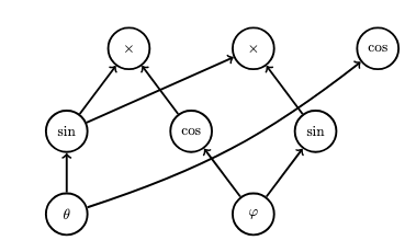
We represent this graph as a function

\[F(\theta,\varphi) = g \circ f\]

which is the composition of the following functions (where we again have chosen one function per level of the graph):

• \(f(\theta, \varphi) = (\sin \theta, \cos \varphi, \sin \varphi, \theta)\),
• \(g(y_1, y_2, y_3, y_4) = (y_1 \cdot y_2, y_1 \cdot y_3, \cos y_4)\).

Note the dummy output \(\theta\) in the fourth component of the output of \(f\), which is used because the parameter \(\theta\) is used in a later level of the graph; this represents the propagation of the value along to later layers.

The Jacobian product is as follows:

\begin{align}J_p(g \circ f) &= \begin{bmatrix}
\frac{\partial g^1}{\partial y_1}(f(p)) & \frac{\partial g^1}{\partial y_2}(f(p)) & \frac{\partial g^1}{\partial y_3}(f(p)) & \frac{\partial g^1}{\partial y_4}(f(p)) \\
\frac{\partial g^2}{\partial y_1}(f(p)) & \frac{\partial g^2}{\partial y_2}(f(p)) & \frac{\partial g^2}{\partial y_3}(f(p)) & \frac{\partial g^2}{\partial y_4}(f(p)) \\
\frac{\partial g^3}{\partial y_1}(f(p)) & \frac{\partial g^3}{\partial y_2}(f(p)) & \frac{\partial g^3}{\partial y_3}(f(p)) & \frac{\partial g^3}{\partial y_4}(f(p))
\end{bmatrix} \\&\times \begin{bmatrix}
\frac{\partial f^1}{\partial \theta}(p) & \frac{\partial f^1}{\partial \varphi}(p) \\
\frac{\partial f^2}{\partial \theta}(p) & \frac{\partial f^2}{\partial \varphi}(p) \\
\frac{\partial f^3}{\partial \theta}(p) & \frac{\partial f^3}{\partial \varphi}(p) \\
\frac{\partial f^4}{\partial \theta}(p) & \frac{\partial f^4}{\partial \varphi}(p) \\
\end{bmatrix}
\end{align}

The partial derivatives are computed as follows (where \(p=(\theta,\varphi)\)):

• \(\frac{\partial f^1}{\partial \theta}(p) = \cos \theta\),
• \(\frac{\partial f^2}{\partial \varphi}(p) = -\sin \varphi\),
• \(\frac{\partial f^3}{\partial \varphi}(p) = \cos \varphi\),
• \(\frac{\partial f^4}{\partial \theta}(p) = 1\),
• \(\frac{\partial g^1}{\partial y_1}(f(p)) = \cos \varphi\),
• \(\frac{\partial g^1}{\partial y_2}(f(p)) = \sin \theta\),
• \(\frac{\partial g^2}{\partial y_1}(f(p)) = \sin \varphi\),
• \(\frac{\partial g^2}{\partial y_3}(f(p)) = \sin \theta\),
• \(\frac{\partial g^3}{\partial y_4}(f(p)) = -\sin \theta\).

The final matrix is

\[\begin{bmatrix}
\cos \theta \cos \varphi & -\sin \theta \sin \varphi \\
\cos \theta \sin \varphi & \sin \theta \cos \varphi \\
-\sin \theta & 0
\end{bmatrix}.\]

Consider the term at row \(1\) and column \(1\) of this matrix:

\[\frac{\partial g^1}{\partial y_1}(f(p)) \cdot \frac{\partial f^1}{\partial \theta}(p) + \frac{\partial g^1}{\partial y_2}(f(p)) \cdot \frac{\partial f^2}{\partial \theta}(p) + \frac{\partial g^1}{\partial y_3}(f(p)) \cdot \frac{\partial f^3}{\partial \theta}(p) + \frac{\partial g^1}{\partial y_4}(f(p)) \cdot \frac{\partial f^4}{\partial \theta}(p).\]

There is only one non-zero term in this sum:

\[\frac{\partial g^1}{\partial y_1}(f(p)) \cdot \frac{\partial f^1}{\partial \theta}(p) = \cos \theta \cos \varphi.\]

Consider the following crucial observations:

• There are 5 paths from sinks to sources.
• The entry at row \(3\), column \(2\) is \(0\) since there is no path from the \(\cos\) node to the \(\varphi\) node.
• Every term in the resultant matrix is a sum of products of partial derivatives, where each term in the sum represents a path and each factor each product represents an intermediate node along this path.

Example

Consider one final example of backpropagation. Consider the following graph:

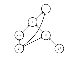
This graph represents the function

\[F(x^1,x^2) = \sin x^1 + x^1 \cdot x^2 + x^1.\]

The function \(F\) can be expressed as the composite

\[F = h \circ g \circ f\]

of the following functions (one per level of the graph):

• \(f(x^1,x^2) = (\sin x^1, x^1 \cdot x^2, x^1)\),
• \(g(y^1, y^2,y^3) = (y^1 + y^2, y^3)\),
• \(h(z^1,z^2) = z^1 + z^2\).

The Jacobian matrix \(J_pF\) (where \(p = (x^1, x^2)\)) is computed from the following product:

\begin{align}\begin{bmatrix}J_pF &= \frac{\partial h}{\partial z^1}(g(f(p))) & \frac{\partial h}{\partial z^2}(g(f(p)))\end{bmatrix} \\& \times \begin{bmatrix}\frac{\partial g^1}{\partial y^1}(f(p)) & \frac{\partial g^1}{\partial y^2}(f(p)) & \frac{\partial g^1}{\partial y^3}(f(p)) \\ \frac{\partial g^2}{\partial y^1}(f(p)) & \frac{\partial g^2}{\partial y^2}(f(p)) & \frac{\partial g^2}{\partial y^3}(f(p)) \end{bmatrix} \\& \times \begin{bmatrix}\frac{\partial f^1}{\partial x^1}(p) & \frac{\partial f^1}{\partial x^2}(p) \\ \frac{\partial f^2}{\partial x^1}(p) & \frac{\partial f^2}{\partial x^2}(p) \\ \frac{\partial f^3}{\partial x^1}(p) & \frac{\partial f^3}{\partial x^2}(p) \end{bmatrix}.\end{align}

The values of these matrices are computed as follows:

\[J_pF = \begin{bmatrix}1 & 1\end{bmatrix}\begin{bmatrix}1 & 1 & 0 \\ 0 & 0 & 1\end{bmatrix}\begin{bmatrix}0 & \cos x^1 \\ x^1 & x^2 \\ 0 & 1\end{bmatrix} = \begin{bmatrix}x^1 & \cos x^1 + x^1 + 1\end{bmatrix}.\]

Consider the following crucial observations:

• Every term in the sum \(\cos x^1 + x^1 + 1\) corresponds to a path from the sink to a source.
• Every term in the sum \(\cos x^1 + x^1 + 1\) is a product of partial derivatives.
• Each partial derivative factor represents one node along the respective path.
• Sums accumulate in source nodes.

The Algorithm

The prior examples of backpropagation indicate the following key properties:

• Every term in the Jacobian matrix is a sum of products of partial derivatives.
• Every summand term within these sums represents a distinct path in the graph from a source to a sink.
• Every summand term within these sums is a product of partial derivative factors.
• Every partial derivative factor within these products represents a node along the respective path.
• The sums accumulate in the source nodes where the paths terminate.

This suggests that we need to traverse every backward path in the graph, computing a product of partial derivatives along the way, one per node along the path, and finally accumulating each such product as a sum within each source node.

The backpropagation algorithm is essentially as follows:

1. Compute the value of the graph. Cache the value of each subgraph at the root of the respective subgraph.
2. For each sink node n, go to step 3 with current_node=n, seed=1, accumulation_index=index(n), where index(n) is the index of n among all the sink nodes (0 for the first, 1 for the second, etc., in any arbitrary but consistent order).
3. If current_node is a source node, set current_node.derivatives[sink_index] += seed and then terminate the current path. Otherwise, go to step 4.
4. For each child node child_node of current_node, compute the partial derivative derivative of the function represented by current_node with respect to the parameter represented by child_node evaluated at the point represented by the value (which may be a vector of values) current_node.values cached at current_node. Go to step 3 with current_node=child_node and seed = seed * derivative.

The following code listing indicates a basic implementation in the Python programming language:

import math

class Node:	
	def __init__(self, id, operation, predecessors=[]):
		self.id = id
		self.operation = operation
		self.predecessors = predecessors
		self.successors = []
		self.derivatives = []
		self.values = None
		for predecessor in predecessors:
			predecessor.successors.append(self)

	def evaluate(self):
		for predecessor in self.predecessors:
			predecessor.evaluate()
		self.value = self.operation.apply(self.predecessor_values())
        
	def forward(self, accumulation_index, id=0, seed=1.0):
		derivative = self.operation.derivative(self.index(id), self.predecessor_values())
		if not self.successors:
			self.accumulate(accumulation_index, seed * derivative)
			return
		for successor in self.successors:
 			successor.forward(accumulation_index, self.id, seed * derivative)
        
	def backward(self, accumulation_index=0, seed=1.0):
		if not self.predecessors:
			self.accumulate(accumulation_index, seed)
			return
		for (index, predecessor) in enumerate(self.predecessors):
			derivative = self.operation.derivative(index, self.predecessor_values())
			predecessor.backward(accumulation_index, seed * derivative)
            
	def accumulate(self, index, derivative):
		if len(self.derivatives) <= index:
			self.derivatives.extend([0.0] * (index - len(self.derivatives) + 1))
		self.derivatives[index] += derivative
        
	def index(self, id):
		return next((index for index, node in enumerate(self.predecessors) if node.id == id), 0)
        
	def predecessor_values(self):
		return list(map(lambda node: node.value, self.predecessors))

	def __add__(self, other):
		return Node(Node.next_id(), Add(), [self, other])
        
	def __mul__(self, other):
		return Node(Node.next_id(), Mul(), [self, other])
        
	@staticmethod
	def next_id():
		i = Node.counter
		Node.counter = Node.counter + 1
		return i
        
class Op:
	def apply(self, values):
		pass
	def derivative(self, index):
		pass
        
class Mul(Op):
	def apply(self, values):
		return values[0] * values[1]
	def derivative(self, index, values):
		if index == 0:
			return values[1]
		elif index == 1:
			return values[0]
        
class Add(Op):
	def apply(self, values):
		return values[0] + values[1]
	def derivative(self, index, values):
		return 1.0
        
class Sin(Op):
	def apply(self, values):
		return math.sin(values[0])
	def derivative(self, index, values):
		return math.cos(values[0])

class Cos(Op):
	def apply(self, values):
		return math.cos(values[0])
	def derivative(self, index, values):
		return -math.sin(values[0])
        
class Var(Op):
	def __init__(self, value):
		self.value = value
	def apply(self, values):
		return self.value
	def derivative(self, index, values):
		return 1.0

def val(value):
	return Node(Node.next_id(), Var(value))
    
def sin(n):
	return Node(Node.next_id(), Sin(), [n])
    
def cos(n):
	return Node(Node.next_id(), Cos(), [n])

This code can be used, for example, as follows:

v1 = val(2.0)
v2 = val(3.0)
v = sin(v1) + v1*v2 + v1
v.evaluate()
v.backward()
print(v.value)
print(v1.derivatives)
print(v2.derivatives)

When executed, this prints the following output:

8.909297426825681
[3.5838531634528574]
[2.0]

Differentiable Programming

Most deep learning frameworks, such as the popular PyTorch library, enable differentiable programming, which is the systematic use of a technique called automatic differentiation to compute the derivatives (i.e., their representation as Jacobian matrices) of differentiable programs (i.e., programs which model differentiable functions \(f : \mathbb{R}^n \rightarrow \mathbb{R}^m\). The backpropagation algorithm can then be applied to arbitrary computational graphs represented by source programs. There are many ways that automatic differentiation can be implemented; for instance, in the example program above, operator overloading was used to define arithmetic operations on nodes, so that, for instance, it is possible to write

v1 = val(2.0)
v2 = val(3.0)
v = sin(v1) + v1*v2 + v1

Most deep learning frameworks use tensors, which are simply multi-dimensional arrays (which are unrelated to the mathematical concept of a tensor) as a basic concept. One can define tensors and apply various operations to them which construct (either explicitly or implicitly) a (possibly dynamic) computational graph which can then be optimized and executed in various fashions (e.g. on one or more GPUs).

Differentiable programming obviates the need for programmers to explicitly compute derivatives, which can be tedious and error prone, especially when changes are applied to the program. Furthermore, differentiable programming enables efficient execution of optimization algorithms (for instance, by parallel execution on GPUs).

See the following post on differentiable programming for more information.

The Training Process

We will now summarize the overall training process. The summary will present the logical process at a high-level; the actual details may vary.

1. A corpus consisting of many individual texts is compiled from various sources (e.g. Wikipedia, etc.).
2. The texts are tokenized. These tokenized texts are concatenated together with special end-of-text token delimiters interspersed between them. For technical reasons, some implementations may require padding to ensure that texts have a common length. The corpus is divided into samples (sequences of tokens) of the chosen context window length, where each sample is separated by the chosen stride. Samples are grouped into batches. These batches are shuffled in order to randomize them (for stochastic gradient descent).
3. For each batch, its samples (sequences of tokens) are input into the model, which outputs a corresponding sequence of probability distributions over the token vocabulary.
4. Each sample (sequence of tokens) is shifted by a stride of one token to determine the targets (supervisory labels) of each subsequence. The respective targets and estimated probability distributions are input into the cross-entropy loss (which is estimated over each batch).
5. Backpropagation is performed in order to compute the gradient with respect to the batch.
6. The model parameters are updated using the computed gradients by applying some form of adaptive gradient descent.

The process then continues with the next batch, until all batches are processed. The batches may be re-shuffled again and the entire process may start over. Each iteration through the batches is called an epoch.

This is illustrated in the following figure:

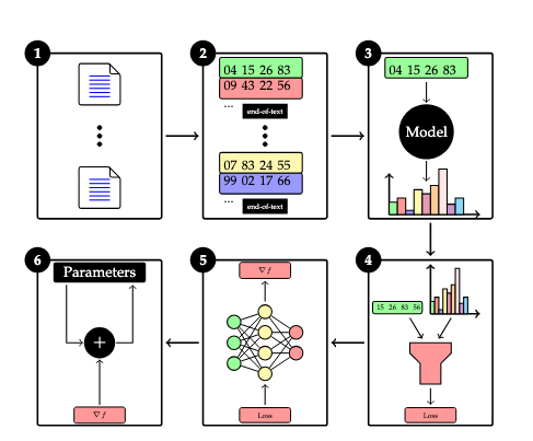
Text Generation

The model is capable of producing one word at a time in response to a prompt. To produce larger responses, a technique called autoregression is applied. The first word produced is appended to the original prompt, defining an augmented prompt, which is then input into the model to product another word, and so on, and so forth.

1. Alice was beginning to \(\rightarrow\) get
2. Alice was beginning to get \(\rightarrow\) very
3. Alice was beginning to get very \(\rightarrow\) tired
4. etc.

References

Reference [1] describes the original GPT concept. Reference [2] describes the GPT-2 model. Reference [3] describes the GPT-3 model. Reference [4] introduces the self-attention mechanism.

1. Radford, Alec; Narasimhan, Karthik; Salimans, Tim; Sutskever, Ilya (June 11, 2018). "Improving Language Understanding by Generative Pre-Training" (PDF). OpenAI. Archived (PDF).
2. Radford, Alec; Wu, Jeffrey; Child, Rewon; Luan, David; Amodei, Dario; Sutskever, Ilua (14 February 2019). "Language models are unsupervised multitask learners" (PDF). OpenAI. Archived 
3. Brown, Tom B.; Mann, Benjamin; Ryder, Nick; Subbiah, Melanie; Kaplan, Jared; Dhariwal, Prafulla; Neelakantan, Arvind; Shyam, Pranav; Sastry, Girish; Askell, Amanda; Agarwal, Sandhini; Herbert-Voss, Ariel; Krueger, Gretchen; Henighan, Tom; Child, Rewon; Ramesh, Aditya; Ziegler, Daniel M.; Wu, Jeffrey; Winter, Clemens; Hesse, Christopher; Chen, Mark; Sigler, Eric; Litwin, Mateusz; Gray, Scott; Chess, Benjamin; Clark, Jack; Berner, Christopher; McCandlish, Sam; Radford, Alec; Sutskever, Ilya; Amodei, Dario (May 28, 2020). "Language Models are Few-Shot Learners". arXiv:2005.14165.
4. Vaswani, Ashish; Shazeer, Noam; Parmar, Niki; Uszkoreit, Jakob; Jones, Llion; Gomez, Aidan N; Kaiser, Łukasz; Polosukhin, Illia (2017). "Attention is All you Need" (PDF). Advances in Neural Information Processing Systems. 30. Curran Associates, Inc.

Further Reading

The book Build a Large Language Model (from Scratch) is a helpful resource which describes how to implement an LLM using PyTorch.