Monads in Computer Science
This post explores the concept of a monad in computer science and its expression in various programming languages.


Monads are a well-established component of modern functional programming. Although they are most conspicuously used in the programming language Haskell, they can be used in other programming languages, and they have been implicitly adopted in Java 8 via the Stream interface and Optional class. This post attempts to explain the precise relationship between the mathematical concept of a monad, some of its applications in theoretical computer science, and its manifestation in various programming languages while supplying all of the necessary mathematical background along the way.
Introduction
The mathematical concept of a monad was applied in theoretical computer science by Eugenio Moggi in order to provide a categorical semantics for computations in his seminal papers [1] and [2].
Notions of Computation
Monads abstract notions of computation, i.e., kinds or sorts of computations. Common examples of such notions of computation include the following:
- Partial Computations (i.e., computations that might not yield any value)
- Stateful Computations
- Transactional Computations
- Exception-raising Computations
- Nondeterministic Computations
- I/O (Side-effecting) Computations
- Continuation-Passing Style Computations
- Parallel Computations
- Distributed Computations
- Asynchronous Computations
Typically, such notions of computation are merely implicit from the context of the source code of a programming language. However, monads differ in that they expressly represent various notions of computation as formal first-class types and related functions of the programming language.
Categorical Semantics
Definition (Category). A category consists of:
- A collection of objects usually denoted \(A\), \(B\), \(C\), etc.,
- A collection of arrows (a.k.a. morphisms) usually denoted \(f\), \(g\), \(h\), etc.,
- For each arrow \(f\), objects \(\mathrm{dom}(f)\) and \(\mathrm{cod}(f)\), the domain and codomain of \(f\), respectively, where we write \(f : A \rightarrow B\) to indicate that \(\mathrm{dom}(f) = A\) and \(\mathrm{cod}(f) = B\),
- For each pair of compatible arrows \(f : A \rightarrow B\) and \(g : B \rightarrow C\) (i.e. \(\mathrm{cod}(f) = \mathrm{dom}(g)\)), an arrow \(g \circ f : A \rightarrow C\) called the composite of \(g\) and \(f\) (often read "\(g\) after \(f\)"),
- For each object \(A\) an arrow \(1_A : A \rightarrow A\) called the identity arrow on \(A\).
These items must satisfy the following two axioms:
- For all \(f : A \rightarrow B\), \(g : B \rightarrow C\), \(h : C \rightarrow D\), \((h \circ g) \circ f = h \circ (g \circ f)\) (i.e. composition is associative),
- For all \(f : A \rightarrow B\), \(f \circ 1_A = f = 1_B \circ f\) (i.e. the identity arrows act as units with respect to composition).
We say that the category is small if both its collection of objects and its collection of arrows are sets. If, for any two objects \(A\) and \(B\) of a category \(\mathcal{C}\), the collection of arrows \(A \rightarrow B\) comprises a set, then we say that the category is locally small. In any locally small category, we can define a set \(\mathrm{Hom}_{\mathcal{C}}(A,B)\) called the hom-set (since morphisms generalize homomorphisms), which consists of the set of all arrows \(A \rightarrow B\).
The opposite category \(\mathcal{C}^{op}\) of a category \(\mathcal{C}\) is the same as \(\mathcal{C}\), yet with all of the arrows formally inverted.
Definition (Opposite Category). Given a category \(\mathcal{C}\), its opposite category \(\mathcal{C}^{op}\) is defined such that:
- The objects of \(\mathcal{C}^{op}\) are the objects of \(\mathcal{C}\),
- An arrow \(f : A \rightarrow B\) in \(\mathcal{C}^{op}\) is an arrow \(f : B \rightarrow A\) in \(\mathcal{C}\), i.e., \(\mathrm{Hom}_{\mathcal{C}^{op}}(A,B) = \mathrm{Hom}_{\mathcal{C}}(B,A)\) .
Writing \(f'\) for the arrow in \(\mathcal{C}^{op}\) that corresponds to the same arrow \(f\) in \(\mathcal{C}\) and \(A'\) for the object in \(\mathcal{C}^{op}\) that corresponds to the same object \(A\) in \(\mathcal{C}\) in order to formally distinguish them, we therefore have the following equivalences:
- \(\mathrm{dom}(f') = \mathrm{cod}(f)\) and \(\mathrm{cod}(f') = \mathrm{dom}(f)\),
- \(1_C' = (1_C)'\),
\(f' \circ g' = (g \circ f)'\), i.e., a diagram such as the following in \(\mathcal{C}^{op}\)
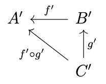
corresponds to the following diagram in \(\mathcal{C}\)
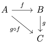
i.e., a diagram commutes in \(\mathcal{C}^{op}\) if and only if its "dual'' diagram commutes in \(\mathcal{C}\).
The Semantic Category
We can associate with any programming language a category \(\mathcal{C}\) whose objects are the types of the programming language and whose morphisms are functions (or programs) between types.
For each type \(A\) we associate a type \(TA\) which represents the "\(T\)-computations of type \(A\)", i.e. those computations of notion \(T\) that yield a value of type \(A\). The type \(T\) is a unary type constructor and thus a type of the programming language; it is a mapping \(A \mapsto TA\) from types to types that takes a type \(A\) as input and produces a related type \(TA\) as output. It can be conceived as a parameterized type or a decoration of a type. There is thus a distinction between the type \(A\) and computations of type \(A\), i.e., \(TA\).
Elements
To represent set membership categorically (using the morphisms of \(\mathbf{Set}\), i.e., functions), observe that a function \(f\) from a singleton set \(1 = \{*\}\) (a set with exactly one element) to a set \(A\) is equivalent to an element (i.e. the set \(A^{1}\) is isomorphic to \(A\)). Intuitively, such a function selects an element of \(A\), namely \(f(*)\). Thus, in the category \(\mathbf{Set}\), elements of a set \(A\) can be represented as morphisms \(1 \rightarrow A\). We say that a set \(A\) is _completely determined_ by its elements \(1 \rightarrow A\) since for any set \(B\), \(\mathrm{Hom}(1,A) \cong \mathrm{Hom}(1,B) \equiv A \cong B\) in direct analogy with the axiom of extensionality.
There is exactly one function from any set to a singleton set. In any category, an object \(1\) such that for any other object \(A\) there is a unique morphism \(A \rightarrow 1\) is called a terminal object.
Definition (Terminal Object). An object \(1\) of a category \(\mathcal{C}\) is a terminal object if for every object \(A\) of \(\mathcal{C}\), there exists a unique arrow \(A \rightarrow 1\).
We might suggest this as a categorification of the concept of "element" in other categories; however, there are two principal problems: first of all, the category might not have a terminal object. Second, even if it does possess a terminal object, objects might not be completely determined by their elements. However, as a corollary of the Yoneda Lemma, every object \(A\) is completely determined by the morphisms \(X \rightarrow A\) from all objects \(X\) into \(A\), that is \(\mathrm{Hom}(-,A) \cong \mathrm{Hom}(-,B) \equiv A \cong B\). Thus, we may adopt arbitrary morphisms \(X \rightarrow A\) as generalized elements.
Definition (Generalized Element). A generalized element of an object \(A\) in a category \(\mathcal{C}\) is an arrow \(e : X \rightarrow A\) for some object \(X\) of \(\mathcal{C}\).
Therefore, a program that performs a \(T\)-computation and yields a value of type \(B\) can be modeled as a generalized element of \(TB\), e.g. a morphism \(A \rightarrow TB\).
The Kleisli Category
In order to model such programs, we introduce an additional category \(\mathcal{C_{T}}\) whose objects are the objects of the semantic category \(\mathcal{C}\) but whose morphisms are \(T\)-type programs, i.e. a morphism \(A \rightarrow B\) in \(\mathcal{C_{T}}\) is a morphism \(A \rightarrow TB\) in \(\mathcal{C}\).
Composition
Now we want to consider exactly what conditions we must impose upon \(\mathcal{C}\) for \(\mathcal{C_{T}}\) to be a category. First of all, we must be able to define composition in \(\mathcal{C_{T}}\). Two morphisms \(f : A \rightarrow B\) and \(g : B \rightarrow C\) in \(\mathcal{C_{T}}\) correspond to morphisms \(f : A \rightarrow TB\) and \(g : B \rightarrow TC\) in \(\mathcal{C}\). These morphisms are incompatible since \(\mathrm{cod}(f) \not = \mathrm{dom}(g)\). However, given our interpretation of the category \(\mathcal{C}\) as a category of types of a programming language, we can easily _extend_ or _lift_ \(g\) to a morphism \(g^{*} : TA \rightarrow TB\) as follows: the lifting \(g^{*}\) intuitively represents a program that executes a \(T\)-computation of type \(A\), extracts the result of type \(A\), and then applies it to \(g\) to produce a \(T\)-computation of type \(B\). Thus, we require that the category \(\mathcal{C}\) have a mapping \(\_^{*}\) that maps any morphism of the form \(f : A \rightarrow TB\) to a corresponding morphism of the form \(f^{*} : TA \rightarrow TB\), and we define composition \(g \circ_{T} f\) in \(\mathcal{C_{T}}\) to be \(g^{*} \circ f\).
Identities
Next, we must define identity morphisms in \(\mathcal{C_{T}}\). An identity morphism \(1_A : A \rightarrow A\) in \(\mathcal{C_{T}}\) corresponds to a morphism \(\eta_A : A \rightarrow TA\) in \(\mathcal{C}\). Thus, we require that there exist a morphism \(\eta_A : A \rightarrow TA\) for every object \(A\) of \(\mathcal{C}\). For any morphism \(f : A \rightarrow B\) in \(\mathcal{C_{T}}\), it must be the case that \(f \circ_{T} 1_A = f = 1_B \circ_{T} f\). By definition, \(f \circ_{T} 1_A = f^{*} \circ \eta_A\). Thus, we require that \(f^{*} \circ \eta_A = f\). Again, by definition, \(1_B \circ f = \eta_B^{*} \circ f\). In order that \(\eta_B^{*} \circ f = f\), we require that \(\eta_B^{*} = 1_{TB}\).
Associativity
Finally, we must ensure the associativity of morphisms in \(\mathcal{C_{T}}\). This means that for any morphisms \(f : A \rightarrow B\), \(g : B \rightarrow C\), and \(h : C \rightarrow D\), \((h \circ_{T} g) \circ_{T} f = h \circ_{T} (g \circ_{T} f)\). Expanding this by its definition, it must be the case that \((h^{*} \circ g)^{*} \circ f = h^{*} \circ (g^{*} \circ f)\). If \((h^{*} \circ g)^{*} = h^{*} \circ g^{*}\), then this is guaranteed, since we can then reduce this expression to \((h^{*} \circ g^{*}) \circ f = h^{*} \circ (g^{*} \circ f)\), which is guaranteed since \(\mathcal{C}\) is a category.
Kleisli Triples
Thus, we've derived the requirements summarized in the following definition.
Definition (Kleisli Triple). A Kleisli triple is a triple \((T,\eta,\_^{*})\) where:
- \(T : \mathrm{Obj}(\mathcal{C}) \rightarrow \mathrm{Obj}(\mathcal{C})\) is an object map ,
- \(\eta_A : A \rightarrow TA\) for every object \(A\) of \(\mathcal{C}\),
- \(f^{*} : TA \rightarrow TA\) for every morphism \(f : A \rightarrow TA\) of \(\mathcal{C}\).
Furthermore, the following conditions must be satisfied:
- \(\eta_A^{*} = 1_{TA}\) for all objects \(A\) of \(\mathcal{C}\),
- \(f^{*} \circ \eta_A = f\) for all morphisms \(f : A \rightarrow TB\) of \(\mathcal{C}\),
- \((g^{*} \circ f)^{*} = g^{*} \circ f^{*}\) for all morphisms \(f : A \rightarrow TB\) and \(g : B \rightarrow TC\) of \(\mathcal{C}\).
Kleisli triples are named after the mathematician Heinrich Kleisli who first investigated such triples. The associated category \(\mathcal{C_{T}}\) is called the Kleisli Category.
Definition (Kleisli Category).
Given a category \(\mathcal{C}\) and a Kleisli triple \((T,\eta,\_^*)\), the associated Kleisli category \(\mathcal{C_T}\) is defined as follows:
- The objects of \(\mathcal{C_T}\) are the objects of \(\mathcal{C}\),
- An arrow \(f : A \rightarrow B\) in \(\mathcal{C_T}\) is an arrow \(f : A \rightarrow TB\) in \(\mathcal{C}\), i.e. \(\mathrm{Hom}_{\mathcal{C_T}}(A,B) = \mathrm{Hom}_{\mathcal{C}}(A,TB)\),
- The composition \(g \circ_{\mathcal{C_T}} f\) of arrows \(f : A \rightarrow B\) and \(g : B \rightarrow C\) in \(\mathcal{C_T}\) is defined as \(g^* \circ f\),
- The identity arrow \(1_A\) on each object \(A\) in \(\mathcal{C_T}\) is \(\eta_A\).
As it turns out, Kleisli triples are presentations of an abstract concept known as a monad.
Extending \(T\) to a Functor
A functor is a homomorphism of categories, i.e., a structure-preserving mapping of the objects and arrows of one category to the objects and arrows of another category. Specifically, a functor preserves domains, codomains, identity arrows, and composition, taking commutative diagrams to commutative diagrams.
Definition (Functor). A functor \(F : \mathcal{C} \rightarrow \mathcal{D}\) is a mapping of objects to objects (e.g., \(A \mapsto FA\)) and arrows to arrows (e.g., \(f \mapsto Ff\)) from a category \(\mathcal{C}\) to a category \(\mathcal{D}\) such that:
- \(F(f : A \rightarrow B) : FA \rightarrow FB\) (i.e. \(F\) preserves domains and codomains),
- \(F1_A = 1_{FA}\) (i.e. \(F\) preserves identity arrows),
- \(F(g \circ f) = Fg \circ Ff\) for all \(f\), \(g\) in \(\mathcal{C}\) (i.e. \(F\) preserves composition) .
Such functors are also called covariant functors. A contravariant functor is a functor that reverses arrows.
Definition (Contravariant Functor). A _contravariant_ functor \(F\) is a functor \(F : \mathcal{C}^{op} \rightarrow \mathcal{D}\). This entails the following:
- \(F(f : A \rightarrow B) : FB \rightarrow FA\) for \(f\) in \(\mathcal{C}\),
- \(F(g \circ f) = Ff \circ Fg\) for \(f\) and \(g\) in \(\mathcal{C}\).
Note that a contravariant functor \(F\) can also be considered a functor \(F : \mathcal{C}^{op} \rightarrow \mathcal{D}\).
\(T\) is an object map; it is natural to ask if we can extend it to a functor, i.e., if we can define \(Tf : TA \rightarrow TB\) for arbitrary morphisms \(f : A \rightarrow B\). Indeed, there is only one choice: \(Tf = (\eta_B \circ f)^{*}\). To confirm that \(T\) preserves composition, note that for any \(f : A \rightarrow B\) and \(g : B \rightarrow C\) the following equality holds,
\begin{split}T(g \circ f) & = (\eta_C \circ (g \circ f))^{*} \\& = ((\eta_C \circ g) \circ f)^{*} \\& = (((\eta_C \circ g)^{*} \circ \eta_B) \circ f)^{*} \\& = ((\eta_C \circ g)^{*} \circ (\eta_B \circ f))^{*} \\& = (\eta_C \circ g)^{*} \circ (\eta_B \circ f)^{*} \\& = Tg \circ Tf,\end{split}
and to confirm that \(T\) preserves identities, note that for any identity morphism \(1_A : A \rightarrow A\), the following equality holds.
\begin{split}T(1_A) & = (\eta_A \circ 1_A)^{*} \\& = \eta_A^{*} \\& = 1_{TA}.\end{split}
The Algebraic Structure around \(T\)
We now examine the algebraic structure that attends the functor \(T\).
Monoids
The lifting \(1_{TA}^* : TTA \rightarrow TA\) resembles a multiplication, and the arrow \(\eta_A : A \rightarrow TA\) resembles a unit, i.e. there is an apparent monoidal structure, which we describe in detail below.
Definition (Monoid). A monoid is a triple \((M,m,e)\) consisting of a set \(M\), a closed binary operation \(m\) (i.e. a function \(m : M \times M \rightarrow M\)), and a distinguished element \(e \in M\) such that the following axioms hold (where we simply write \(ab\) instead of \(m(a,b)\)):
- \(ea = a = ae\) for all \(a \in M\) (\(e\) is the unit for \(m\)),
- \((ab)c = a(bc)\) for all \(a,b,c \in M\) (\(m\) is associative).
Monoids in \(\mathbf{Set}\)
We can define a monoid categorically, i.e., purely in terms of objects and morphisms in \(\mathbf{Set}\) without reference to elements as follows:
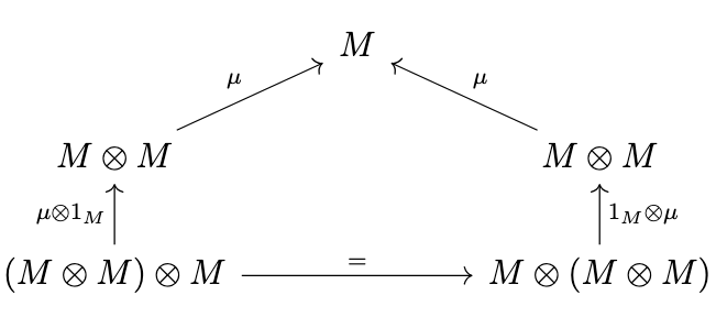
Definition (Monoid). A monoid is a set \(M\) together with a function \(m : M \times M \rightarrow M\) and a function \(e: 1 \rightarrow M\) (where \(1\) is any singleton set) such that the following diagrams commute.
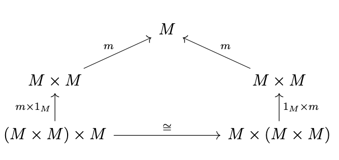
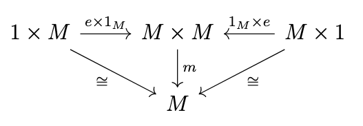
The "pentagon" diagram expresses associativity, whereas the "triangle" diagram expresses unitality. The product \(A \times B\) of two sets \(A\) and \(B\) is the usual cartesian product \(A \times B = \{(a,b) \mid a \in A \land b \in B\}\). The isomorphism denoted \(\cong\) in the pentagon represents the associator \(\alpha : (M \times M) \times M \rightarrow M \times (M \times M)\), i.e. the canonical isomorphism \(((a,b),c) \mapsto (a,(b,c))\) and the isomorphisms denoted \(\cong\) in the triangle diagram represent the left unitor \(\lambda : 1 \times M \rightarrow M\) and right unitor \(\rho : M \times 1 \rightarrow M\), i.e. the canonical isomorphisms \((*,a) \mapsto a\) and \((a,*) \mapsto a\), respectively. The product of two functions \(f : A \rightarrow A'\) and \(g : B \rightarrow B'\) is the function \(f \times g : A \times B \rightarrow A' \times B'\) defined such that \((f \times g) (a,b) = (f(a),g(b))\).
Thus, the pentagon diagram states that \(m((m \times 1_M)((a,b),c)) = m((1_M \times M)(\alpha((a,b),c)))\), i.e. that \((ab)c = a(bc)\) and the triangle diagram states that \(m((e \times 1_M)(*,a)) = \lambda(*,a)\) and \(m((1_M \times e)(a,*)) = \rho(a,*)\), i.e. that \(ea = a\) and \(ae = a\), respectively.
Strict Monoidal Categories
There is a heuristic principle in category theory known as the microcosm principle which states that we can define a structure of some type within a category which somehow possesses a version of the very same structure. The category \(\mathbf{Set}\) is in fact a monoidal category; for our purposes, however, we will only require the much simpler concept of a strict monoidal category.
Definition (Strict Monoidal Category). A strict monoidal category is a category \(\mathcal{M}\) together with a closed binary operation (i.e., bifunctor) \(\otimes : \mathcal{M} \times \mathcal{M} \rightarrow \mathcal{M}\) and distinguished object \(I\) of \(\mathcal{M}\) such that for any objects \(A,B,C\) of \(\mathcal{M}\), \((A \otimes B) \otimes C = A \otimes (B \otimes C)\) and \(I \otimes A = A = I \otimes A\).
Thus, there is a straightforward analogy between the definition of a monoid and strict monoidal category. The strict monoidal category of interest is the category \(\mathrm{End}(\mathcal{C})\) of endofunctors on a category \(\mathcal{C}\) since we are studying the endofunctor \(T\). This is a strict monoidal category if we let \(\otimes = \circ\) and \(I\) be the identity functor since for any endofunctor \(T\), \((T \circ T) \circ T = T \circ (T \circ T)\) and \(I \circ T = T = T \circ I\).
Monoids in Strict Monoidal Categories
We can define a monoid in a strict monoidal category by generalizing the diagrams above, replacing \(\times\) with \(\otimes\).
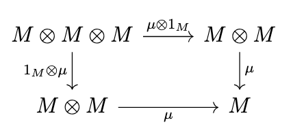
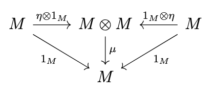
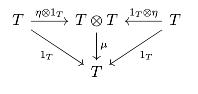
Definition (Monoid in a Strict Monoidal Category). A monoid in a strict monoidal category \(\mathcal{M}\) is an object \(M\) of \(\mathcal{M}\) together with a multiplication \(\mu : M \otimes M \rightarrow M\) and unit \(\eta : 1 \rightarrow M\) such that the following diagrams commute.
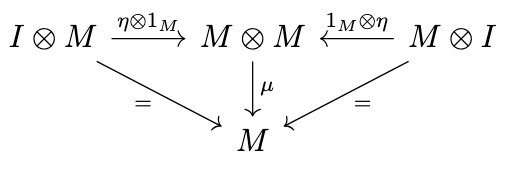
Note, however, that since the isomorphisms have become identities and \(M \otimes I = M\), we can simplify these diagrams as follows.
Natural Transformations
Our goal is to apply this definition to the category \(\mathrm{End}(\mathcal{C})\). However, we must first define the \emph{morphisms} of this category, i.e. we must define a \emph{morphism between functors}.
Let \(F : \mathcal{C} \rightarrow \mathcal{D}\) and \(G : \mathcal{C} \rightarrow \mathcal{D}\) be functors. The image of each functor in \(\mathcal{D}\) is what distinguishes the functors. Thus, a mapping of functors maps the image of one functor onto the image of the other. Since the image of each functor is a category (i.e. a subcategory of \(\mathcal{D}\)), this mapping is essentially a functor; however, it is important that this mapping not be an \emph{arbitrary} functor, but that the mapping exist \emph{in the context of \(\mathcal{D}\)}, i.e. that it be comprised of morphisms of \(\mathcal{D}\)}. Like a functor, it maps objects to objects and morphisms to morphisms, but \emph{via morphisms of \(\mathcal{D}\)}.
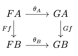
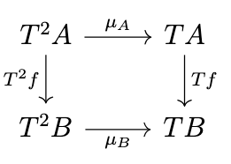
Definition (Natural Transformation). A natural transformation is a family of morphisms \(\theta_A : FA \rightarrow GA\), one for each object \(A\) of \(\mathcal{C}\), such that for any morphism \(f : A \rightarrow B\) in \(\mathcal{C}\), the following diagram commutes, i.e., \(Gf \circ \theta_A = \theta_B \circ Ff\). Each morphism \(\theta_A\) is called the component of \(\theta\) at \(A\)}.
Composition of Natural Transformations
Next, we must define the composition of natural transformations. There are two standard ways to compose natural transformations. The first (which we refer to hereafter simply as "composition") is performed by composing the components of each natural transformation.
Definition (Composition of Natural Transformations). Given functors \(F_1 : \mathcal{C} \rightarrow \mathcal{D}\), \(F_2 : \mathcal{C} \rightarrow \mathcal{D}\) and \(F_3 : \mathcal{C} \rightarrow \mathcal{D}\) and natural transformations \(\alpha : F_1 \rightarrow F_2\) and \(\beta : F_2 \rightarrow F_3\), we define a natural transformation \(\beta \circ \alpha\) such that \((\beta \circ \alpha)_A : F_1 \rightarrow F_3\) as \(\beta_A \circ \alpha_A\) for each object \(A\) of \(\mathcal{C}\) as in the following diagram.
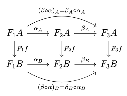
This is always a natural transformation, by the following equations.
\begin{split}(\beta \circ \alpha)_B \circ F_1f & = \beta_B \circ \alpha_B \circ F_1f \\& = \beta_B \circ F_2f \circ \alpha_A \\& = F_3f \circ \beta_A \circ \alpha_A \\& = F_3f \circ (\beta \circ \alpha)_A\end{split}
Product of Natural Transformations
There is another standard way to compose natural transformations, called the product of natural transformations, which is performed by composing the underlying functors and then deriving a natural transformation, i.e., by "superimposing" the respective diagrams. Let \(F_1\), \(G_1\) be functors from \(\mathcal{C}\) to \(\mathcal{D}\) and \(F_2\), \(G_2\) be functors from \(\mathcal{D}\) to \(\mathcal{E}\) and let \(\alpha : F_1 \rightarrow G_1\) and \(\beta : F_2 \rightarrow G_2\) be two natural transformations as in the following diagrams.
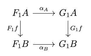
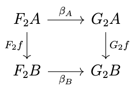
We want to define the natural transformation \(\beta * \alpha : F_2F_1 \rightarrow G_2G_1\), as in the following diagram.
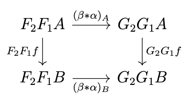
There are two ways to define this, and both are equal; we can work from "the outside in" or "the inside out", i.e. we can change \(F_2F_1\) into \(G_2G_1\) by first changing \(F_2\) into \(G_2\) and then changing \(F_1\) into \(G_1\), or vice versa, as in the following diagram.
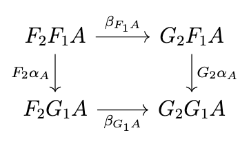
Definition (Product of Natural Transformations). Let \(F_1\), \(G_1\) be functors from \(\mathcal{C}\) to \(\mathcal{D}\) and \(F_2\), \(G_2\) be functors from \(\mathcal{D}\) to \(\mathcal{E}\) and let \(\alpha : F_1 \rightarrow G_1\) and \(\beta : F_2 \rightarrow G_2\) be two natural transformations. The product \(\beta * \alpha\) is the natural transformation defined such that \((\beta * \alpha)_A = G_2\alpha \circ \beta_{F_1A} = \beta_{G_1A} \circ F_2\alpha_A\). These two expressions are equivalent since \(\beta\) is a natural transformation and thus the previous diagram commutes.
To confirm that \(\beta * \alpha\) so defined is indeed a natural transformation, note the following equivalences.
\begin{split}(\beta * \alpha)_B \circ F_2F_1f & = G_2\alpha_B \circ \beta_{F_1B} \circ F_2F_1f \\& = G_2\alpha_B \circ G_2F_1f \circ \beta_{F_1A} \\& = G_2(\alpha_B \circ F_1f) \circ \beta_{F_1A} \\& = G_2(G_1f \circ \alpha_A) \circ \beta_{F_1A} \\& = G_2G_1f \circ G_2\alpha_A \circ \beta_{F_1A} \\& = G_2G_1f \circ (\beta * \alpha)_A\end{split}
The Category \(\mathrm{End}(\mathcal{C})\)
Thus, we are now prepared to define the category \(\mathrm{End}(\mathcal{C})\).
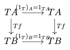
Definition (The Category \(\mathrm{End}(\mathcal{C})\)). For a category \(\mathcal{C}\), the category \(\mathrm{End}(\mathcal{C})\) is the category whose objects are endofunctors \(T : \mathcal{C} \rightarrow \mathcal{C}\), and whose morphisms are natural transformations between these endofunctors; the identities are the identity natural transformations \(1_T : T \rightarrow T\), and composition is the composition of natural transformations. The identity natural transformation is defined as in the following diagram.
Monoids in \(\mathrm{End}(\mathcal{C})\)
Now we are finally able to define a monoid object in the category \(\mathrm{End}(\mathcal{C})\); let \(\otimes\) be defined as follows:
- \(T_2 \otimes T_1 = T_2 \circ T_1\) for endofunctors \(T_1\) and \(T_2\),
- \(\beta \otimes \alpha = \beta * \alpha\) for natural transformations \(\alpha : T_1 \rightarrow T_2\) and \(\beta : T_2 \rightarrow T_3\).
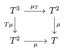
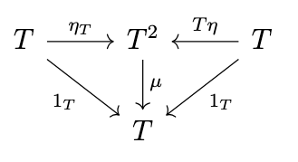
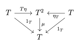
That is, the tensor product \(\otimes\) is the composition of endofunctors and the product of natural transformations. A monoid is then given by the following diagrams.
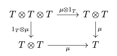
Now, we write \(\mu_T\) for \(\mu \otimes 1_T\), \(T\mu\) for \(1_T \otimes \mu\), i.e. we define the composition of a natural transformation and a _functor_ to be the composition of the natural transformation with the respective identity transformation on that functor. Likewise, we write \(\eta_T\) for \(\eta * 1_T\) and \(T\eta\) for \(1_T * \eta\). Writing \(T^2\) for \(T \circ T\) and \(T^3\) for \(T \circ T \circ T\), the previous diagrams are equivalent to the following diagrams.
Monads
A monoid in the strict monoidal category \(\mathrm{End}(\mathcal{C})\) is precisely what a monad is. Thus, we have the following definition:
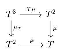
Definition (Monad). A monad is a triple \((T,\eta,\mu)\) consisting of an endofunctor \(T\) on a category \(\mathcal{C}\), a natural transformation \(\eta : 1_{\mathcal{C}} \rightarrow T\), and a natural transformation \(\mu : T^2 \rightarrow T\) such that the previous two diagrams commute.
Kleisli Triples and Monads
In this section, we demonstrate the equivalence of Kleisli triples and monads.
Kleisli Triples Induce Monads
We demonstrate that Kleisli triples induce monads. Given a Kleisli triple \((T,\eta,\_^*)\), we can define a corresponding monad \((T,\eta,\mu)\) where \(\mu=1_{TA}^*\).
Naturality of Kleisli \(\eta\)
First, we want to confirm that the \(\eta\) of the Kleisli triple is a natural transformation \(\eta : I \rightarrow T\) from the identity functor \(I\) to the functor \(T\), that is, that the following diagram commutes.
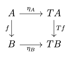
This is indeed the case, as demonstrated by the following equations.
\begin{split}\eta_B \circ f & = (\eta_B \circ f)^{*} \circ \eta_A \
& = Tf \circ \eta_A\end{split}
Naturality of Kleisli \(\mu\)
We also want to confirm that \(\mu\) as defined previously (\(\mu_A = 1_{TA}^*\)) is also a natural transformation \(\mu : T^2 \rightarrow T\), i.e., that the following diagram commutes.
Note the following equivalences.
\begin{split}\mu_B \circ T^{2}f & = 1_{TB}^{*} \circ T((\eta_B \circ f)^{*}) \\& = 1_{TB}^{*} \circ (\eta_{TB} \circ (\eta_B \circ f)^{*})^{*} \\& = (1_{TB}^{*} \circ \eta_{TB} \circ (\eta_B \circ f)^{*})^{*} \\& = (1_{TB} \circ (\eta_B \circ f)^{*})^{*} \\& = (\eta_B \circ f)^{**} \\& = ((\eta_B \circ f)^{*} \circ \eta_A)^{**} \\& = ((\eta_B \circ f)^{*} \circ \eta_A^{*})^{*} \\& = (\eta_B \circ f)^{*} \circ \eta_A^{**} \\& = (\eta_B \circ f)^{*} \circ 1_{TA}^{*} \\& = Tf \circ \mu_A\end{split}
Unitality of Kleisli \(\eta\)
To confirm that the Kleisli \(\eta\) is unital, i.e., that the following diagram commutes,
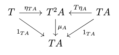
note the following equivalences.
\begin{split}(\mu \circ T\eta)_A & = \mu_A \circ T\eta_A \\& = 1_{TA}^* \circ (\eta_{TA} \circ \eta_A)^* \\& = (1_{TA}^* \circ \eta_{TA} \circ \eta_A)^* \\& = (1_{TA} \circ \eta_A)* \\& = \eta_{TA}^* \\& = 1_{TA} \\& = 1_{TA}^* \circ \eta_{TA} \\& = \mu_A \circ \eta_{TA} \\& = (\mu \circ {\eta}T)_A\end{split}
Associativity of Kleisli \(\mu\)
To confirm that the Kleisli \(\mu\) is associative, i.e., that the following diagram commutes,
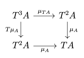
note the following equivalences.
\begin{split}(\mu \circ T\mu)_A & = \mu_A \circ (T\mu)_A \\& = \mu_A \circ T\mu_A \\& = 1_{TA}^* \circ T(1_{TA}^*) \\& = 1_{TA}^* \circ (\eta_{TA} \circ 1_{TA}^*)^* \\& = (1_{TA}^* \circ \eta_{TA} \circ 1_{TA}^*)^* \\& = (1_{TA} \circ 1_{TA}^*)^* \\& = 1_{TA}^{**} \\& = (1_{TA}^* \circ 1_{T^2A})^* \\& = 1_{TA}^* \circ 1_{T^2A}^* \\& = \mu_A \circ \mu_{TA} \\& = (\mu \circ {\mu}T)_A\end{split}
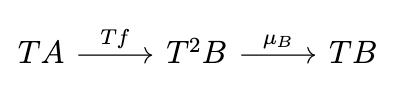
Monads Induce Kleisli Triples
Given a monad \((T, \eta, \mu)\), we can define the corresponding Kleisli triple \((T, \eta, \_^*)\) where \(f^* = \mu_B \circ Tf\) for \(f : A \rightarrow B\) as in the following diagram.
Kleisli Unit Laws
We must verify that the Kleisli unit laws hold for the induced Kleisli triple. Note the following equivalences.
\begin{split}\eta_A^* & = \mu_A \circ T\eta_A \\& = 1_{TA}.\end{split}
\begin{split}f^* \circ \eta_A & = \mu_B \circ Tf \circ \eta_A \\& = \mu_B \circ \eta_{TB} \circ f \\& = \mu_B \circ (T\eta)_B \circ f \\& = 1_{TB} \circ f \\& = f.\end{split}
Finally, we must verify that the conditions imposed upon Kleisli composition hold for the induced Kleisli triple. Note the following equivalences.
\begin{split}(g^* \circ f)^* & = \mu_C \circ T(g^* \circ f) \\& = \mu_C \circ Tg^* \circ Tf \\& = \mu_C \circ T(\mu_C \circ Tg) \circ Tf \\& = \mu_C \circ T\mu_C \circ T^2g \circ Tf \\& = \mu_C \circ Tg \circ \mu_B \circ Tf \\& = g^* \circ f^*\end{split}
Thus, monads and Kleisli triples are equivalent. However, in programming languages, Kleisli triples are typically used to define monads since their associated functions and rules are easier to state and verify and since Kleisli composition has an intuitive computational interpretation.
The Kleisli Adjunction
By definition, there is a one-to-one correspondence between morphisms \(A \rightarrow B\) in the Kleisli category \(\mathcal{C_T}\) and morphisms \(A \rightarrow TB\) in the semantic category \(\mathcal{C}\), i.e. \(\mathrm{Hom}_{\mathcal{C_T}}(A,B) = \mathrm{Hom}_{\mathcal{C}}(A,TB)\) as shown in the following figure.
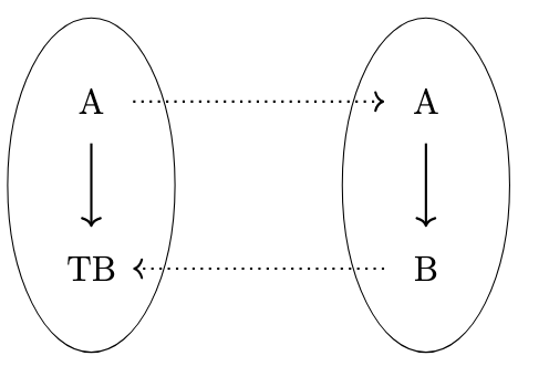
The dotted lines in the previous figure indicate that the connection between these morphisms is mediated by a pair of functors, as shown in the following figure.
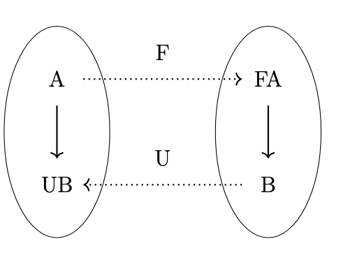
We can define a functor \(F : \mathcal{C} \rightarrow \mathcal{C_T}\) as follows:
- \(FA = A\) for all objects \(A\) of \(\mathcal{C}\),
- \(Ff = \eta_B \circ f\) for all morphisms \(f : A \rightarrow B\) of \(\mathcal{C}\),
To confirm that this is indeed a functor, note that for any identity morphism \(1_A\) and morphisms \(f : A \rightarrow B\) and \(g : B \rightarrow C\) in \(\mathcal{C}\), the following equations hold.
\begin{split}F1_A & = \eta_A \circ 1_A \\& = \eta_A \\& = 1_{FA} \end{split}
\begin{split}F(g \circ f) & = \eta_C \circ (g \circ f) \\& = (\eta_C \circ g) \circ f \\& = (\eta_C \circ g)^* \circ \eta_B \circ f \\& = (\eta_C \circ g) \circ_{\mathcal{C_T}} (\eta_B \circ f) \\& = Fg \circ_{\mathcal{C_T}} Ff\end{split}
Likewise, we can also define a functor \(U : \mathcal{C_T} \rightarrow \mathcal{C}\) as follows:
- \(UA = TA\) for all objects \(A\) of \(\mathcal{C_T}\),
- \(Uf = f^*\) for all morphisms \(f\) of \(\mathcal{C_T}\).
To confirm that this is indeed a functor, note that for any identity morphism \(1_A\) and morphisms \(f : A \rightarrow B\) and \(g : B \rightarrow C\) in \(\mathcal{C_T}\), the following equations hold.
\begin{split}U1_A & = U\eta_A \\& = \eta_A^* \\& = 1_{TA} \\& = 1_{UA}\end{split}
\begin{split}U(g \circ_{\mathcal{C_T}} f) & = (g \circ_{\mathcal{C_T}} f)^* \\& = (g^* \circ f)^* \\& = g^* \circ f^* \\& = Ug \circ Uf\end{split}
Adjoint Functors
Functors \(F : \mathcal{C} \rightarrow \mathcal{D}\) and \(U : \mathcal{D} \rightarrow \mathcal{C}\) are a pair of adjoint functors if \(\mathrm{Hom}_{\mathcal{D}}(FC,D) \cong \mathrm{Hom}_{\mathcal{C}}(C,UD)\) and this isomorphism is natural in both \(C\) and \(D\). We write \(F \dashv U\) and say that \(F\) is left adjoint to \(U\) and \(U\) is right adjoint to \(F\).
These hom-sets induce hom-functors, i.e. \(\mathrm{Hom}_{\mathcal{C_T}}(F-,-) : \mathcal{C} \times \mathcal{C_T} \rightarrow \mathbf{Set}\) and \(\mathrm{Hom}_{\mathcal{C}}(-,U-) : \mathcal{C} \times \mathcal{C_T} \rightarrow \mathbf{Set}\). These two functors are naturally isomorphic, i.e., there is a natural isomorphism \(\phi : \mathrm{Hom}_{\mathcal{C_T}}(F-,-) \rightarrow \mathrm{Hom}_{\mathcal{C}}(-,U-)\). In order to interpret what this means, we need to examine some basic properties of such functors. Later on we will discuss a purely equational definition of adjoint functors.
Bifunctors
These functors are called bifunctors because they map pairs of objects.
Given two categories \(\mathcal{C}\) and \(\mathcal{D}\), we can form their product category.
Definition (Product Category).
For categories \(\mathcal{C}\) and \(\mathcal{D}\), the product category \(\mathcal{C \times D}\) is the category defined as follows:
- Objects are pairs of objects \((C,D)\) with \(C\) in \(\mathcal{C}\) and \(D\) in \(\mathcal{D}\),
- Arrows are pairs of arrows \((f,g) : (C,D) \rightarrow (C',D')\) with \(f : C \rightarrow C'\) in \(\mathcal{C}\) and \(g : D \rightarrow D'\) in \(\mathcal{D}\),
- Composition is done component-wise, i.e. \((f',g') \circ (f,g) = (f' \circ f, g' \circ g)\),
- The identity on \((C,D)\) is \((1_C,1_D)\).
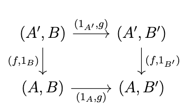
A bifunctor is then a functor from a product category to another category. Let us consider a bifunctor \(F : \mathcal{C}^{op} \times \mathcal{C} \rightarrow D\). Given any arrow \((f,g) : (A,B) \rightarrow (A',B')\) in \(\mathcal{C}^{op} \times \mathcal{C}\), this arrow corresponds to an arrow \((f,g) : (A',B) \rightarrow (A,B')\) in \(\mathcal{C} \times \mathcal{C}\), and it factors as \((f,g) = (1_A,g) \circ (f,1_B) = (f,1_{B'}) \circ (1_{A'},g)\), i.e., the following diagram commutes.
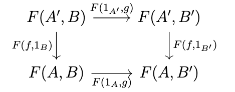
Since \(F\) is a functor, the following diagram also commutes in \(\mathcal{D}\).
Thus, there are four induced functors:
- \(F(-,B) : \mathcal{C}^{op} \rightarrow \mathcal{D}\), \(F(f,B) = F(f,1_B)\),
- \(F(-,B') : \mathcal{C}^{op} \rightarrow \mathcal{D}\), \(F(f,B') = F(f,1_B')\),
- \(F(A',-) : \mathcal{C} \rightarrow \mathcal{D}\), \(F(A',g) = F(1_{A'},g)\),
- \(F(A,-) : \mathcal{C} \rightarrow \mathcal{D}\), \(F(A,g) = F(1_A,g)\).
We can think of these as parameterized functors. Furthermore, the commutativity of the previous diagram also implies that there are two natural transformations:
- \(F(-,g) : F(-,B) \rightarrow F(-,B')\), \(F(-,g)_A = F(A,g) = F(1_A,g)\),
- \(F(f,-) : F(A',-) \rightarrow F(A,-)\), \(F(f,-)_B = F(f,B) = F(f,1_B)\).
Conversely, given such "parameterized" functors, we can construct a corresponding bifunctor using the previous diagram. A natural transformation \(\theta\) between bifunctors \(F : \mathcal{C}^{op} \times \mathcal{C} \rightarrow \mathcal{D}\) is a family of arrows that makes the following diagram commute.
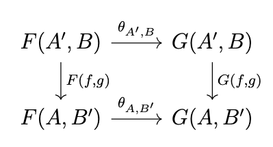
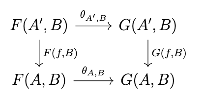
Now, suppose that if we hold \(B\) constant (that is, we let \(g\) be the identity \(1_B\)) then the functor \(F(-,B)\) is naturally equivalent to the functor \(G(-,B)\) via the family of arrows \(\theta\), i.e., that the following diagram commutes.
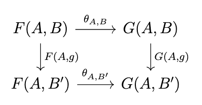
Suppose further that if we hold \(A\) constant (that is, we let \(f\) be the identity \(1_A\)) that the functor \(F(A,-)\) is naturally equivalent to the functor \(G(A,-)\) via the family of arrows \(\theta\), i.e., that the following diagram commutes.
Putting these previous diagrams together yields the following composite diagram.
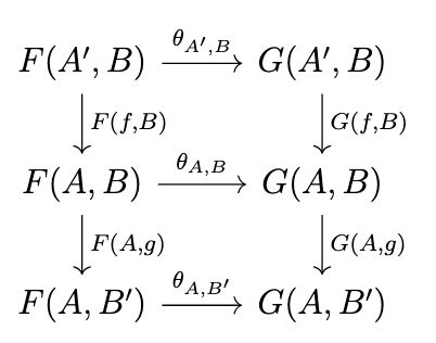
In other words, we have the equivalences specified as follows.
\begin{split}\theta_{A,B'} \circ F(f,g) &= \theta_{A,B'} \circ F(A,g) \circ F(f,B) \\& = G(A,g) \circ \theta_{A,B} \circ F(f,B) \\&= G(A,g) \circ G(f,B) \circ \theta_{A',B} \\& = G(f,g) \circ \theta_{A',B}.\end{split}
Thus, if we independently establish that the family of arrows \(\theta\) makes \(F(A,-)\) and \(G(A,-)\) naturally equivalent and \(F(-,B)\) and \(G(-,B)\) naturally equivalent, then this suffices to demonstrate that \(\theta\) is a natural transformation from \(F\) to \(G\).
Hom-Functors
Next, let us consider an example of such a bifunctor; in a locally-small category \(\mathcal{C}\) the notion of hom-set induces a corresponding hom-functor \(\mathrm{Hom}_{\mathcal{C}}(-,-) : \mathcal{C}^{op} \times \mathcal{C} \rightarrow \mathbf{Set}\). Given an arrow \(g : B \rightarrow B'\) in \(\mathcal{C}\), for any arrow \(h : A \rightarrow B\), we can produce an arrow \(g \circ h : A \rightarrow B'\), as indicated in the following diagram.
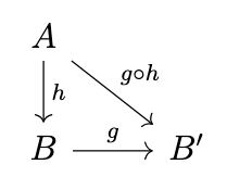
Thus, we can produce a functor \(\mathrm{Hom}_{\mathcal{C}}(A,-) : \mathcal{C} \rightarrow \mathbf{Set}\) where \(\mathrm{Hom}_{\mathcal{C}}(A,g)(h) = g \circ h\). Likewise, given an arrow \(f : A \rightarrow A'\) in \(\mathcal{C}\), for any arrow \(h : A' \rightarrow B\), we can produce an arrow \(h \circ f : A \rightarrow B\), as indicated in the following diagram.
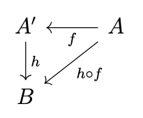
Thus, we can produce a functor \(\mathrm{Hom}_{\mathcal{C}}(-,B) : \mathcal{C}^{op} \rightarrow \mathbf{Set}\) where \(\mathrm{Hom}_{\mathcal{C}}(f,B)(h) = h \circ f\), i.e. a contravariant functor. As we established previously, we can assemble these functors into a bifunctor.
Naturality in \(A\)
Returning to the Kleisli adjunction outlined above, we wish to establish that the isomorphism \(\mathrm{Hom}_{\mathcal{C_T}}(F-,-) \cong \mathrm{Hom}_{\mathcal{C}}(-,U-)\) is natural. If we fix one of the bifunctor's arguments, then we produce a functor, e.g. fixing \(B\) produces \(\mathrm{Hom}_{\mathcal{C_T}}(F-,B)\) and \(\mathrm{Hom}_{\mathcal{C}}(-,UB)\) and fixing \(A\) produces \(\mathrm{Hom}_{\mathcal{C_T}}(FA,-)\) and \(\mathrm{Hom}_{\mathcal{C}}(A,U-)\). Naturality in \(A\) means that the following diagram commutes for any \(f : A \rightarrow A'\) in \(\mathcal{C}\).
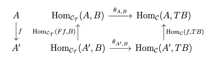
Note that for any \(x \in \mathrm{Hom}_{\mathcal{C_T}}(A',B)\), the following equation holds.
\begin{split}(\theta_{A,B} \circ \mathrm{Hom}_{\mathcal{C_T}}(Ff,B))(x) & = \mathrm{Hom}_{\mathcal{C_T}}(Ff,B)(x) \\& = x \circ_{\mathcal{C_T}} Ff \\& = x^* \circ Ff \\& = x^* \circ \eta_B \circ f \\& = x \circ f \\& = \mathrm{Hom}_{\mathcal{C}}(f,TB)(x) \\& = (\mathrm{Hom}_{\mathcal{C}}(f,TB) \circ \theta_{A',B})(x)\end{split}
Naturality in \(B\)
Naturality in \(B\) means that the following diagram commutes for any \(g : B \rightarrow B'\) in \(\mathcal{C}\).
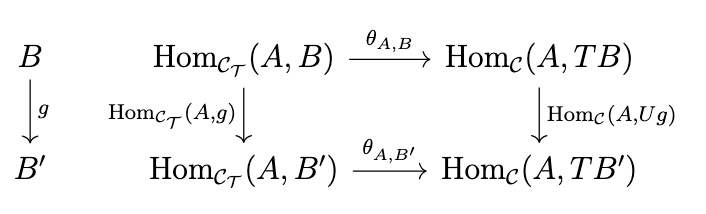
Note that for any \(y \in \mathrm{Hom}_{\mathcal{C_T}}(A,B)\), we have the following equivalences.
\begin{split}(\theta_{A,B'} \circ \mathrm{Hom}_{\mathcal{C_T}}(A,g))(y) & = \mathrm{Hom}_{\mathcal{C_T}}(A,g)(y) \\& = g \circ_{\mathcal{C_T}} y \\& = g^* \circ y \\& = Ug \circ y \\& = \mathrm{Hom}_{\mathcal{C}}(A,Ug)(y) \\& = (\mathrm{Hom}_{\mathcal{C}}(A,Ug) \circ \theta_{A,B})(y)\end{split}
The Unit of an Adjunction
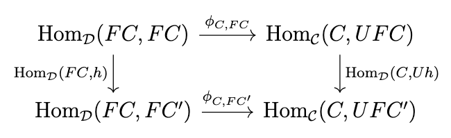
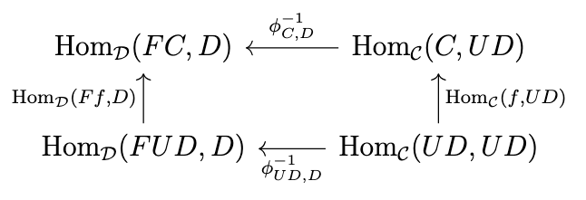
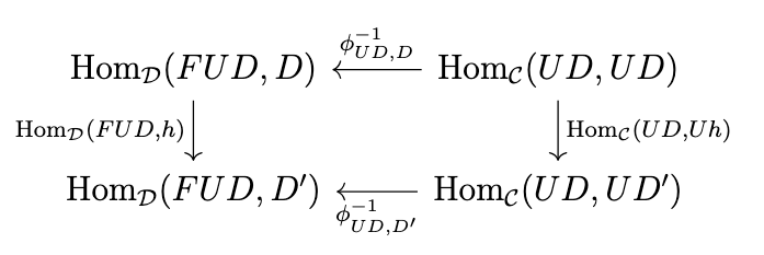
Let \(F \dashv U\) be any adjunction with \(F : \mathcal{C} \rightarrow \mathcal{D}\) and \(U : \mathcal{D} \rightarrow \mathcal{C}\). Naturality in \(D\) means that the following diagram commutes.
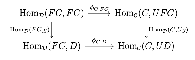
This means that \((\phi_{C,D} \circ \mathrm{Hom}_{\mathcal{D}}(FC,g))(1_{FC}) = (\mathrm{Hom}_{\mathcal{C}}(C,Ug) \circ \phi_{C,FC})(1_{FC})\), which simplifies to \(\phi_{C,D}(g) = Ug \circ \phi_{C,FC}(1_{FC})\), as shown in the following diagram.
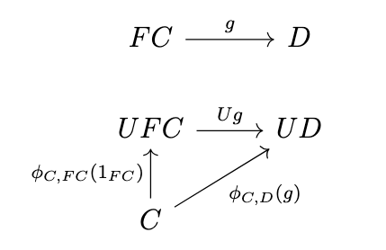
In fact, the morphisms \(\phi_{C,FC}(1_{FC}) : C \rightarrow UFC\) comprise a natural transformation, which we call \(\eta : 1_{\mathcal{C}} \rightarrow UF\), with component \(\eta_C\) shown in the following diagram.
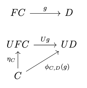
Thus, \(\phi_{C,D}(g) = Ug \circ \eta_C\). To demonstrate that \(\eta\) is natural, we need to show that the following diagram commutes.
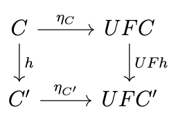
In other words, we must show that \(\eta_{C'} \circ h = UFh \circ \eta_C\). Naturality in \(D\) means that the following diagram commutes.
This means that, \((\phi_{C,FC'} \circ \mathrm{Hom}_{\mathcal{D}}(FC,Fh))(1_{FC}) = (\mathrm{Hom}_{\mathcal{C}}(U,Fh) \circ \phi_{C,FC})(1_{FC})\), which simplifies to \(\phi_{C,FC'}(Fh) = UFh \circ \phi_{C,FC}(1_{FC})\). Naturality in \(C\) means that the following diagram commutes.
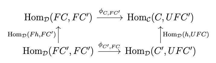
This means that \((\phi_{C,FC'} \circ \mathrm{Hom}_{\mathcal{D}}(Fh,FC'))(1_{FC'}) = (\phi_{C',FC'} \circ \mathrm{Hom}_{\mathcal{C}}(h,UFC))(1_{FC'})\), which simplifies to \(\phi_{C,FC'}(Fh) = \phi_{C',FC'}(1_{FC'}) \circ g\). Combining this equation with the equation \(\phi_{C,FC'}(Fh) = UFh \circ \phi_{C,FC}(1_{FC})\) yields \(\phi_{C,FC'}(Fh) = UFh \circ \phi_{C,FC}(1_{FC})\), which is equivalent to \(\eta_{C'} \circ h = UFh \circ \eta_C\). Thus, \(\eta\) is a natural transformation. Given any \(f : C \rightarrow UD\), since \(\phi\) is an isomorphism and hence bijective, the following diagram commutes if we choose \(g = \phi^{-1}(f)\).
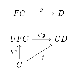
In fact, such a \(g\) is the unique morphism \(FC \rightarrow D\) that makes the the previous diagram commute, since if there were any \(g' : FC \rightarrow D\) such that \(Ug' \circ \eta_C = f\), then since \(\phi_{C,D}(g') = Ug' \circ \eta_C\), it follows that \(\phi_{C,D}(g') = f\) and since \(\phi_{C,D}\) is bijective and \(\phi_{C,D}(g) = f\), it must be the case that \(g = g'\). Thus, we have the following definition.
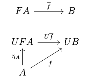
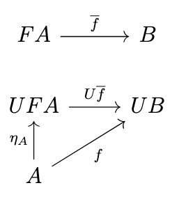
Definition (Unit of an Adjunction). Given an adjunction \(F \dashv U\) with \(F : \mathcal{C} \rightarrow \mathcal{D}\) and \(U : \mathcal{D} \rightarrow \mathcal{C}\), the unit of the adjunction is the natural transformation \(\eta : 1_{\mathcal{C}} \rightarrow UF\) that satisfies the following universal property: for any morphism \(f : A \rightarrow UB\), there exists a unique morphism \(\overline{f} : FA \rightarrow B\) such that \(U\overline{f} \circ \eta_A = f\), i.e., the following diagram commutes:
The Counit of an Adjunction
By naturality in \(C\), the following diagram commutes.
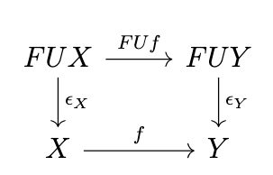
This means that \((\phi^{-1}_{C,D} \circ \mathrm{Hom}_{\mathcal{C}}(f,UD))(1_{UD}) = (\mathrm{Hom}_{\mathcal{D}}(Ff,D) \circ \phi^{-1}_{UD,D})(1_{UD})\), which simplifies to \(\phi^{-1}_{C,D}(f) = \phi^{-1}(1_{UD}) \circ Ff\). The morphisms \(\phi^{-1}_{UD,D}(1_{UD}) : FUD \rightarrow D\) comprise a natural transformation, which we denote \(\epsilon\), with \(\epsilon_D\) shown in the following diagram.
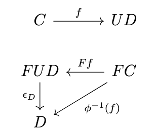
Thus, \(\epsilon_D \circ Ff = \phi^{-1}_{C,D}(f)\). To demonstrate that \(\epsilon\) is natural, we need to show that the following diagram commutes.
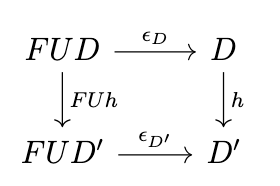
In other words, we must show that \(\epsilon_{D'} \circ FUh = h \circ \epsilon_D\). Naturality in \(C\) means that the following diagram commutes.
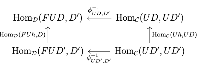
This means that \((\mathrm{Hom}_{\mathcal{D}}(FUh,D) \circ \phi^{-1}_{UD',D'})(1_{UD'}) = (\phi^{-1}_{UD,D'} \circ \mathrm{Hom}_{\mathcal{C}}(Uh,UD'))(1_{UD'})\), which simplifies to \(\epsilon_{D'} \circ FUh = \phi^{-1}_{UD,D'}(Uh)\). Naturality in \(D\) means that the following diagram commutes.
This means that \((\mathrm{Hom}_{\mathcal{D}}(FUD,h) \circ \phi^{-1}_{UD,D})(1_{UD}) = (\phi^{-1}_{UD,D'} \circ \mathrm{Hom}_{\mathcal{C}}(UD,h))(1_{UD})\) which simplifies to \(h \circ \epsilon_D = \phi^{-1}_{UD,D'}(Uh)\). Combining this equation with the equation \(\epsilon_{D'} \circ FUh = \phi^{-1}_{UD,D'}(Uh)\) yields \(\epsilon_{D'} \circ FUh = h \circ \epsilon_D\). Thus, \(\epsilon\) is a natural transformation.
Given any \(f : C \rightarrow UD\), the following diagram commutes if we choose \(g = \phi^{-1}(f)\).
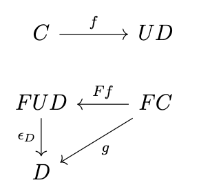
In fact, such an \(f\) is the unique morphism \(C \rightarrow UD\) that makes diagram (\ref{diagram-45}) commute, since if there were any \(f' : C \rightarrow UD\) such that \(\epsilon_D \circ Ff' = g\), then since \(\phi^{-1}_{C,D}(f') = \epsilon_D \circ Ff'\) it follows that \(\phi^{-1}_{C,D}(f') = g\), and since \(\phi^{-1}_{C,D}\) is bijective, it must be the case that \(f = f'\). Thus, we have the following definition.
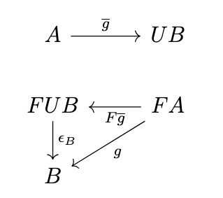
Definition (Counit of an Adjunction). Let \(F \dashv U\) be an adjunction with \(F : \mathcal{C} \rightarrow \mathcal{D}\) and \(U : \mathcal{D} \rightarrow \mathcal{C}\). The counit of the adjunction is the natural transformation \(\epsilon : 1_{\mathcal{D}} \rightarrow FU\) that satisfies the following universal property: for any arrow \(g: FA \rightarrow B\), there exists a unique arrow \(\overline{g} : A \rightarrow UB\) such that \(\epsilon_B \circ F\overline{g} = g\) i.e., the following diagram commutes:
The Triangle Identities
We have derived the following equations:
- \(\phi(g) = Ug \circ \eta_C\) where \(\eta_C = \phi(1_{FC})\),
- \(\phi^{-1}(f) = \epsilon_D \circ Ff\) where \(\epsilon_D = \phi^{-1}(1_{UD})\).
Since \(\phi\) is an isomorphism, we obtain the following equalities as shown in the following diagrams.
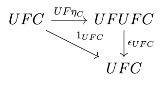
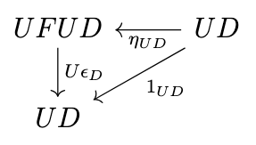
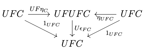
\begin{split}1_{UD} & = \phi(\phi^{-1}(1_{UD})) \\& = U(\phi^{-1}(1_{UD})) \circ \eta_{UD} \\& = U\epsilon_D \circ \eta_{UD}\end{split}
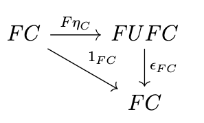
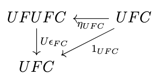
\begin{split}1_{FC} & = \phi^{-1}(\phi(1_{FC})) \\& = \epsilon_{FC} \circ F(\phi(1_{FC})) \\& = \epsilon_{FC} \circ F\eta_C\end{split}
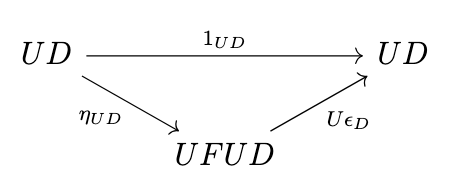
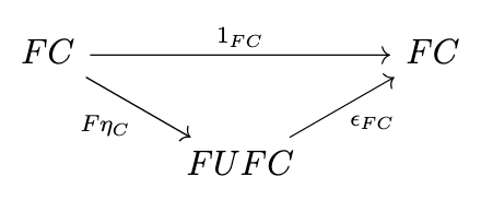
In other words, \(1_U = U\epsilon \circ \eta_U\) and \(1_F = \epsilon_F \circ F\eta\). Together, these equations are known as the triangle identities.
Algebraic Definition of Adjoint Functors
We can stipulate the triangle identities as the definition of an adjunction, since they imply the hom-set definition. This definition has the advantage of being purely equational.
Definition (Adjoint Functors). Functors \(F : \mathcal{C} \rightarrow \mathcal{D}\) and \(U : \mathcal{D} \rightarrow \mathcal{C}\) are adjoint functors if there exist natural transformations \(\eta : 1_C \rightarrow UF\) and \(\epsilon : 1_D \rightarrow FU\) such that \(1_F = \epsilon_F \circ F\eta\) and \(1_U = U\epsilon \circ \eta_U\). We write \(F \dashv U\) and say that \(F\) is left adjoint to \(U\) and \(U\) is right adjoint to \(F\).
We want to establish that this definition implies the universal property of the unit, the universal property of the counit, and the hom-set definition of an adjunction (i.e., for locally-small categories).
First, we establish the universal property of the unit, i.e. that given any arrow \(f : A \rightarrow UB\), there exists a unique arrow \(\overline{f} : FA \rightarrow B\) such that the following diagram commutes, i.e., \(U\overline{f} \circ \eta_A = f\).
Letting \(\overline{f} = \epsilon_B \circ Ff\), we obtain the following equivalences since \(\eta\) is natural.
\begin{split}U(\epsilon_B \circ Ff) \circ \eta_A & = U\epsilon_B \circ UFf \circ \eta_A \\& = U\epsilon_B \circ \eta_{UB} \circ f \\& = 1_{UB} \circ f \\& = f\end{split}
If there is any other arrow \(\overline{\overline{f}}\) such that \(U\overline{\overline{f}} \circ \eta_A = f\), then \(\overline{\overline{f}} = \epsilon_B \circ Ff\) by the following equation.
\begin{split}\epsilon_B \circ Ff & = \epsilon_B \circ F(U\overline{\overline{f}} \circ \eta_A) \\& = \epsilon_B \circ FU\overline{\overline{f}} \circ F\eta_A \\& = \overline{\overline{f}} \circ \epsilon_{FB} \circ F\eta_A \\& = \overline{\overline{f}} \circ 1_{FA} \\& = \overline{\overline{f}}\end{split}
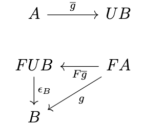
Next, we establish the universal property of the counit, i.e., that given any arrow \(g : FA \rightarrow B\), there exists a unique arrow \(\overline{g} : A \rightarrow UB\) such that the following diagram commutes, i.e., \(\epsilon_B \circ F\overline{g} = g\).
Letting \(\overline{g} = Ug \circ \eta_A\), we obtain the following equivalences since \(\epsilon\) is natural.
\begin{split}\epsilon_B \circ F(Ug \circ \eta_A) & = \epsilon_B \circ FUg \circ F\eta_A \\& = g \circ \epsilon_{FB} \circ F\eta_A \\& = g\end{split}
If there is any other arrow \(\overline{\overline{g}}\) such that \(\epsilon_B \circ F\overline{\overline{g}} = g\), then \(\overline{\overline{g}} = Ug \circ \eta_A\) by the following equation.
\begin{split}Ug \circ \eta_A & = U(\epsilon_B \circ F\overline{\overline{g}}) \circ \eta_A \\& = U\epsilon_B \circ UF\overline{\overline{g}} \circ \eta_A \\& = U\epsilon_B \circ \eta_{UB} \circ \overline{\overline{g}} \\& = 1_{UB} \circ \overline{\overline{g}} \\& = \overline{\overline{g}}\end{split}
Now, assuming that \(\mathcal{C}\) and \(\mathcal{D}\) are locally-small categories, we define a natural isomorphism \(\phi : \mathrm{Hom}_{\mathcal{D}}(F-,-) \rightarrow \mathrm{Hom}_{\mathcal{C}}(-,U-)\) such that \(\phi_{A,B}(g) = Ug \circ \eta_A\) for \(g : FA \rightarrow B\). To confirm that this is an isomorphism, we define its inverse \(\phi^{-1} : \mathrm{Hom}_{\mathcal{C}}(-,U-) \rightarrow \mathrm{Hom}_{\mathcal{D}}(F-,-)\) such that \(\phi^{-1}_{A,B}(f) = \epsilon_B \circ Ff\) for \(f : A \rightarrow UB\). Then \(\phi^{-1}_{A,B}(\phi_{A,B}(g)) = \epsilon_B \circ F(Ug \circ \eta_A) = g\) as established by the above equation and \(\phi_{A,B}(\phi^{-1}_{A,B}(f)) = U(\epsilon_B \circ Ff) \circ \eta_A = f\) as established by the equation above. Naturality in \(A\) means that for any \(h : A' \rightarrow A\), the following diagram commutes,

i.e., \((\phi_{A',B} \circ \mathrm{Hom}_{\mathcal{D}}(Fh,B))(g) = (\mathrm{Hom}_{\mathcal{C}}(h,UB) \circ \phi_{A,B})(g)\) for any \(g : FA \rightarrow B\), which is demonstrated by the following equation.
\begin{split}(\phi_{A',B} \circ \mathrm{Hom}_{\mathcal{D}}(Fh,B))(g) & = \phi_{A',B}(g \circ Fh) \\& = U(g \circ Fh) \circ \eta_{A'} \\& = Ug \circ UFh \circ \eta_{A'} \\& = Ug \circ \eta_A \circ h \\& = \phi_{A,B}(g) \circ h \\& = (\mathrm{Hom}_{\mathcal{C}}(h,UB) \circ \phi_{A,B})(g)\end{split}
Naturality in \(B\) means that for any \(k : B \rightarrow B'\) the following diagram commutes,
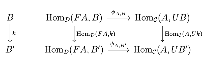
i.e., \((\phi_{A,B'} \circ \mathrm{Hom}_{\mathcal{D}}(FA,k))(g) = (\mathrm{Hom}_{\mathcal{C}}(A,Uk) \circ \phi_{A,B})(g)\) for all \(g : FA \rightarrow B\), which is demonstrated by the following equation.
\begin{split}(\phi_{A,B'} \circ \mathrm{Hom}_{\mathcal{D}}(FA,k))(g) & = \phi_{A,B'}(k \circ g) \\& = U(k \circ g) \circ \eta_A \\& = Uk \circ Ug \circ \eta_A \\& = Uk \circ \phi_{A,B}(g) \\& = (\mathrm{Hom}_{\mathcal{C}}(A,Uk) \circ \phi_{A,B})(g).\end{split}
Adjunctions Induce Monads
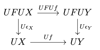
Since \(\epsilon\) is natural, the following diagram commutes for any \(f : X \rightarrow Y\).
If we apply \(U\) to this diagram, then the following diagram commutes.
If we substitute \(\epsilon_{FC}\) for \(f\), then the following diagram commutes.
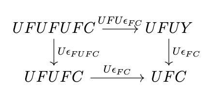
Thus, if we define \(T = UF\), and \(\mu = U\epsilon_F\), then we have the following diagram.
Consider the triangle identity in the following diagram.
If we apply \(U\) to this diagram, we get the following commutative diagram.
Next, consider the triangle identity in the following diagram.
If we substitute \(FC\) for \(D\) in this diagram we obtain the following commutative diagram.
Putting these diagrams together yields the following diagram.
Again, letting \(T = UF\), \(\mu = U\epsilon_F\), we have the following diagram.
Thus, given this adjunction, we can define a monad.
Equivalence of Induced Monads
Now we confirm that, for a Kleisli triple \((T,\eta,\_^*)\), the monad \((\overline{T}=UF,\overline{\eta},\overline{\mu}=U\epsilon_F)\) derived from the Kleisli adjunction \((F,U,\phi,\eta,\epsilon)\) is the same as the monad \((T,\eta,\mu)\) derived directly from the Kleisli triple. First, we demonstrate that the functor \(T\) induced by the Kleisli triple is the same as the functor \(\overline{T}=UF\) derived from the adjunction, as shown in the following equation.
\begin{split}\overline{T}f & = UFf \\& = U(\eta_B \circ f) \\& = (\eta_B \circ f)^* \\& = Tf\end{split}
Next, we demonstrate that the unit \(\eta\) of the adjunction and the unit \(\eta\) of the Kleisli triple coincide in the following equation.
\begin{split}\overline{\eta}_A & = \phi(1_{FA}) \\& = 1_{FA} \\& = 1_A \\& = \eta_A\end{split}
Finally, verify that the natural transformation \(\mu\) derived from the adjunction is the same as the natural transformation defined previously, i.e., \(1_{TA}^*\), as shown in the following equation.
\begin{split}\overline{\mu}_A & = U\epsilon_{FA} \\& = U\epsilon_A \\& = \epsilon_A^* \\& = (\epsilon_A^* \circ \eta_{UA})^* \\& = (U\epsilon_A \circ \eta_{UA})^* \\& = 1_{UA}^* \\& = 1_{TA}^* \\& = \mu_A\end{split}
Examples of Monads in Computer Science
We will now give some examples of common monads used in computer science and functional programming. The key to analyzing each monad is this: a morphism in the Kleisli category corresponds to a morphism of the desired type in the category of types.
The Identity Monad
Given a category \(\mathcal{C}\), the identity monad is the monad \((1_{\mathcal{C}},1_{1_{\mathcal{C}}},1_{1_{\mathcal{C}}})\) where the endofunctor is the identity functor \(1_{\mathcal{C}}\) on \(\mathcal{C}\), and the unit and multiplication are the identity natural transformation \(1_{1_{\mathcal{C}}}\) on the identity functor. This is a trivial example of a monad (i.e., all diagrams commute because they are all comprised of the same identity arrow), but it is useful in many mathematical situations. This monad is not realized in programming languages, which generally use a type constructor to represent monads, and thus the type \(TA\) and the type \(A\) are not identical. However, they are isomorphic.
The Maybe Monad
The maybe monad represents partial computations. The intuitive idea is that we augment a type \(A\) with an additional term \(\bot\) which represents failure, i.e., an incomplete computation. The failure term \(\bot\) inhabits a unit type (i.e. a type with a unique term), which categorically is a terminal object \(1\). We simply combine the original type with the unit type, producing the type \(A + 1\), where \(+\) denotes the coproduct (i.e., sum type).
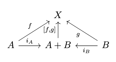
Definition (Coproduct). The coproduct of an object \(A\) and an object \(B\) in a category \(\mathcal{C}\) is an object \(A+B\) together with arrows \(i_A : A \rightarrow A+B\) and \(i_B : B \rightarrow A+B\) called _injections_ such that for any object \(X\) with arrows \(f : A \rightarrow X\) and \(g : B \rightarrow X\), there exists a unique arrow \([f,g] : A+B \rightarrow X\) such that the following diagram commutes, i.e., \([f,g] \circ i_A = f\) and \([f,g] \circ i_B = g\).
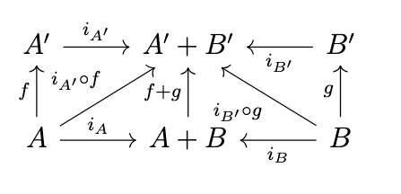
Given coproducts \(A + B\) and \(A' + B'\) and arrows \(f : A \rightarrow A'\) and \(g : B \rightarrow B'\), we can construct an arrow \(f + g : A + B \rightarrow A' + B'\) as \(f+g = [i_{A'} \circ f, i_{B'} \circ g]\) as indicated in the following diagram, i.e., the coproduct is functorial.
Note that in \(\mathbf{Set}\), the coproduct is the disjoint union of sets. We therefore assume that our semantic category has all (small) coproducts. Using the principle stated above, a morphism \(A \rightarrow B\) in the Kleisli category should correspond to a morphism \(A \rightarrow TB\), where \(TB\) represents a partial computation. Thus, we define \(T\) to be the mapping \(X \mapsto X + 1\), i.e.,
- \(TX = X + 1\) for any object \(X\) where \(1\) denotes a terminal object,
- \(Tf = f + 1\) for any morphism \(f\) where \(1\) denotes the identity morphism on the terminal object \(1\).
To confirm that this is a functor, simply note the equivalences in the following equations.
\begin{split}T1_A & = 1_A + 1 \\& = 1_{A + 1} \\& = 1_{TA}\end{split}
\begin{split}T(g \circ f) & = (g \circ f) + 1 \\& = (g + 1) \circ (f + 1) \\& = Tg \circ Tf\end{split}
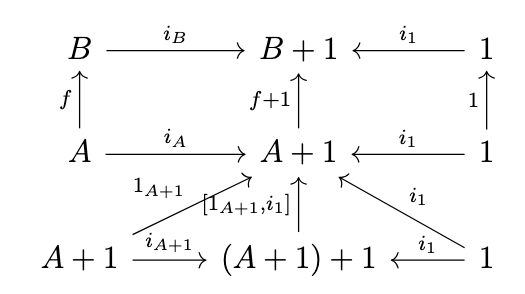
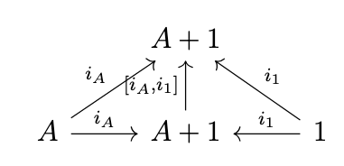
The unit \(\eta\) represents the "inclusion" of values into computations, i.e. a trivial computation. Thus, we define the unit such that \(\eta_A = i_A\) where \(i_A : A \rightarrow A + 1\) denotes the _injection_, which exists by the definition of the coproduct \(A + 1\). For this to be a natural transformation, the following diagram must commute.
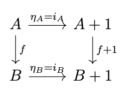
Thus, it must be the case that \(i_B \circ f = (f + 1) \circ i_A\). By definition, \(f + 1 = [i_B \circ f, i_1 \circ 1]\), and by definition of the coproduct, \([i_B \circ f, i_1 \circ 1] \circ i_A = i_B \circ f\), so \(\eta\) is indeed natural.
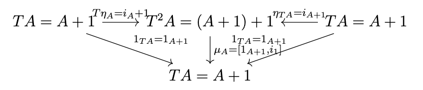
The multiplication \(\mu\) must "join" together two "levels" into a single "level", i.e., \(\mu_A: (A + 1) + 1 \rightarrow A + 1\). By the definition of the coproduct, the following diagram commutes.
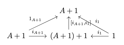
Thus, we define \(\mu_A = [1_{A + 1}, i_1]\). For this to be a natural transformation, the following diagram must commute.
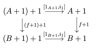
Thus, it must be the case that \([1_{B+1}, i_1] \circ (f + 1) + 1 = (f + 1) \circ [1_{A+1}, i_1]\). Note the following diagram.
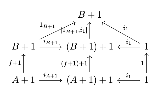
Since \((f + 1) + 1 = [i_{B+1} \circ f + 1,i_1 \circ 1]\) by definition, we have the equivalences in the following equations.
\begin{split}[1_{B+1}, i_1] \circ (f + 1) + 1 \circ 1_{A+1} & = [1_{B+1}, i_1] \circ [i_{B+1} \circ f + 1,i_1 \circ 1] \circ i_{A+1} \\& = [1_{B+1}, i_1] \circ i_{B+1} \circ f + 1 \\& = 1_{B+1} \circ f + 1 \\& = f + 1\end{split}
\begin{split}[1_{B+1}, i_1] \circ (f + 1) + 1 \circ 1_1 & = [1_{B+1}, i_1] \circ [i_{B+1} \circ f + 1,i_1 \circ 1] \circ i_1 \\& = [1_{B+1}, i_1] i_1 \circ 1 \\& = i_1 \circ 1 \\& = i_1\end{split}
By the definition of the coproduct \((A + 1) + 1\), there is a unique morphism \([f + 1, i_1]\) such that \([f + 1, i_1] \circ i_{A+1} = f + 1\) and \([f + 1, i_1] \circ i_1 = i_1\), so it follows that \([1_{B+1}, i_1] \circ (f + 1) + 1 = [f + 1, i_1]\). Next, note the following diagram.
We have the equivalences in the following equations.
\begin{split}f + 1 \circ [1_{A+1},i_1] \circ i_{A+1} & = f + 1 \circ 1_{A+1} \\& = f + 1\end{split}
\begin{split}f + 1 \circ [1_{A+1},i_1] \circ i_1 & = f + 1 \circ i_1 \\& = [i_B \circ f,i_1 \circ 1] \circ i_1 \\& = i_1 \circ 1 \\& = i_1\end{split}
Thus, by the definition of the coproduct \((A + 1) + 1\), it again follows that \(f + 1 \circ [1_{A+1},i_1] = [f + 1, i_1]\). Thus, the required equivalence \([1_{B+1}, i_1] \circ (f + 1) + 1 = (f + 1) \circ [1_{A+1}, i_1]\) holds.
Next, we must verify associativity, i.e., that the following diagram commutes.
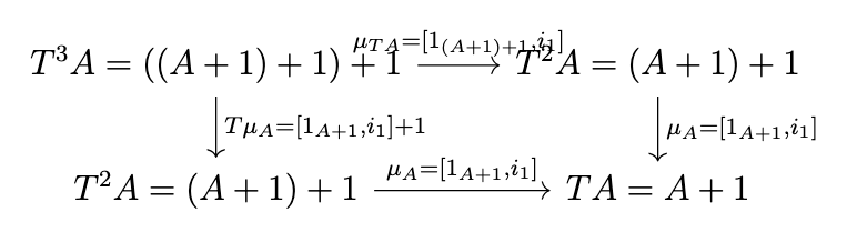
That is, we must verify that \([1_{A+1},i_1] \circ [1_{A+1},i_1] + 1 = [1_{A+1},i_1] \circ [1_{(A+1)+1},i_1]\). Consider the following diagram.
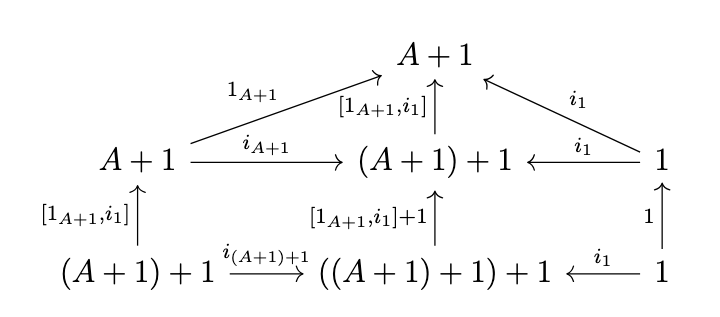
Note the following equivalences.
\begin{split}[1_{A+1},i_1] \circ [1_{A+1},i_1] + 1 \circ i_{(A+1)+1} \\= [1_{A+1},i_1] \circ [i_{A+1} \circ [1_{A+1},i_1],i_1 \circ 1] \circ i_{(A+1)+1} \\= [1_{A+1},i_1] \circ i_{A+1} \circ [1_{A+1},i_1] \\= 1_{A+1} \circ [1_{A+1},i_1] \\= [1_{A+1},i_1]\end{split}
\begin{split}[1_{A+1},i_1] \circ [1_{A+1},i_1] + 1 \circ i_1 \\= [1_{A+1},i_1] \circ [i_{A+1} \circ [1_{A+1},i_1],i_1 \circ 1] \circ i_1 \\= [1_{A+1},i_1] \circ i_1 \\= i_1 \\\end{split}
Thus, by the definition of the coproduct \(((A+1)+1)+1\), it follows that \([1_{A+1},i_1] \circ [1_{A+1},i_1] + 1 = [[1_{A+1},i_1],i_1]\). Next, consider the following diagram.
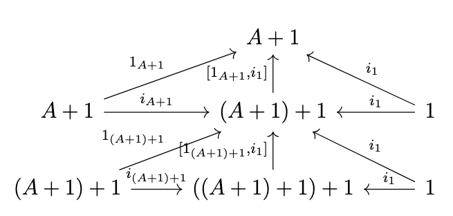
We have the following equivalences.
\begin{split}[1_{A+1},i_1] \circ [1_{(A+1)+1},i_1] \circ i_{(A+1)+1} \\= [1_{A+1},i_1] \circ 1_{(A+1)+1} \\= [1_{A+1},i_1]\end{split}
\begin{split}[1_{A+1},i_1] \circ [1_{(A+1)+1},i_1] \circ i_1 \\= [1_{A+1},i_1] \circ i_1 \\= i_1\end{split}
Thus, by definition of the coproduct \(((A+1)+1)+1\), it follows that \([1_{A+1},i_1] \circ [1_{(A+1)+1},i_1] = [[1_{A+1},i_1],i_1]\). Thus, the associativity diagram is satisfied.
Finally, we must demonstrate that the following diagram commutes.
That is, we must demonstrate that \([1_{A+1},i_1] \circ 1_A + 1 = 1_{A+1}\) and \([1_{A+1},i_1] \circ i_{A+1} = 1_{A+1}\). The latter is immediate. To see the former, note that, by the definition of the coproduct \(A + 1\), there is a unique morphism \([i_A,i_1]\) such that \([i_A,i_1] \circ i_A = i_A\) and \([i_A,i_1] \circ i_1 = i_1\), as indicated in the following diagram.
However, \(1_{A+1}\) is an arrow such that \(1_{A+1} \circ i_A = i_A\) and \(1_{A+1} \circ i_1 = i_1\), so it follows that \([i_A,i_1] = 1_{A+1}\). Thus, we have confirmed that the maybe monad is indeed a monad.
The List Monad
The list monad models nondeterministic computations. The idea is to represent a nondeterministic computation as a collection of potential values rather than a single, definite value. In most functional programming languages, the standard type for representing collections of values is a list.
Mathematically, we model lists as words, i.e., finite sequences of symbols \(a_1a_2\dots a_n\). We will use list notation \([a_1,a_2,\dots,a_n]\) to denote such sequences and refer to words as "lists".
We begin by analyzing the situation in the category \(\mathbf{Set}\). We want to define a monad \((T,\eta,\mu)\). Given a set \(A\), we want \(TA\) to represent all lists \([a_1,a_2,\dots,a_n]\) comprised of elements \(a_i \in A\). This set is sometimes denoted \(A^*\).
The triple \(\overline{A} = (A^*,+,\epsilon)\) forms a monoid where \(+\) denotes list concatenation (i.e. \([a_{1,1},a_{1,2},\dots,a_{1,m}] + [a_{2,1},a_{2,2},\dots,a_{2,n}] = [a_{1,1},a_{1,2},\dots,a_{1,m},a_{2,1},a_{2,2},\dots,a_{2,n}]\)) and \(\epsilon\) denotes the empty list \([]\). Thus, given any set \(A\), we can define a corresponding monoid \(\overline{A}\).
Monoid Homomorphisms
We next define morphisms between monoids.
Definition (Monoid Homomorphism). A monoid homomorphism from a monoid \(\overline{A} = (A,+,\epsilon_A)\) to a monoid \(\overline{B} = (B,+,\epsilon_B)\) is a function \(h : A \rightarrow B\) between the underlying sets \(A\) and \(B\) such that the structure of the monoid is preserved, i.e.,
- \(h(a_1 + a_2) = ha_1 + ha_2\) for all \(a_1,a_2 \in A\),
- \(h(\epsilon_A) = \epsilon_B\).
Free Monoids
In fact, the monoid \(\overline{A} = (A^*,+,\epsilon_A)\) is a canonical example of a so-called free monoid on the set \(A\).
In category theory, to analyze a concept like a free monoid, we analyze it structurally, i.e., according to its morphisms. In particular, we are interested in how a free monoid maps to other monoids; the free monoid should be able to map to any other monoid if we specify a corresponding mapping between the underlying sets of the respective monoids. This is one sense in which it is "free".
Now, consider a free monoid \(FA\) on a set \(A\) and an arbitrary monoid \(B\). We desire that any function \(f : A \rightarrow UB\) (where \(UB\) denotes the underlying set of the monoid \(B\)) induce a homomorphism \(h : FA \rightarrow B\) such that \(h(a_i) = f(a_i)\) for all elements \(a_i \in A\). In order for \(h\) to be a homomorphism, it must be the case that \(h(a_1 + a_2) = h(a_1)+h(a_2)\) for all \(a_1,a_2 \in A\). Thus, \(FA\) cannot, in general, be subject to any extraneous relations such as \(a_1 + a_2 = a_3\), since it might not be the case that \(f(a_1)+f(a_2) = f(a_3)\). This is the sense in which the monoid \(FA\) is free: it is unconstrained by relations (except those that are required by the axioms of a monoid, such as \(a_1\epsilon_A = a_1\)).
Moreover, the free monoid should not contain any elements that are not combinations of the elements of \(A\). This implies that \(h\) is unique since if there were another homomorphism \(h' : FA \rightarrow B\) such that \(h(a_i) = f(a_i)\) for all \(a_i \in A\), then we obtain the following equivalences.
\begin{split}h'([a_1,a_2,\dots,a_n]) & = [h'(a_1),h'(a_2),\dots,h'(a_n)] \\& = [f(a_1),f(a_2),\dots,f(a_n)] \\& = [h(a_1),h(a_2),\dots,h(a_n)] \\& = h([a_1,a_2,\dots,a_n])\end{split}
Since every element of the free monoid \(FA\) is supposed to be such a combination \([a_1,a_2,\dots,a_n]\), it thus follows that \(h' = h\). Thus, we characterize free monoids such that any mapping between the generators \(A\) and the underlying set \(UB\) determines a unique homomorphism \(h : FA \rightarrow B\).
The converse is also true: any homomorphism \(h : FA \rightarrow B\) determines a unique mapping \(f : A \rightarrow UB\) such that \(f(a_i) = h(a_i)\) for all \(a_i \in A\). Thus, there is a one-to-one correspondence between mappings of generators and homomorphisms.
Free-Forgetful Adjunction
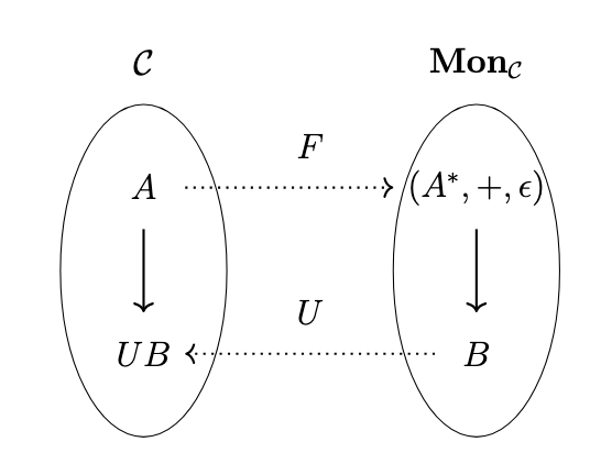
Thus, we have the situation depicted in the following figure.
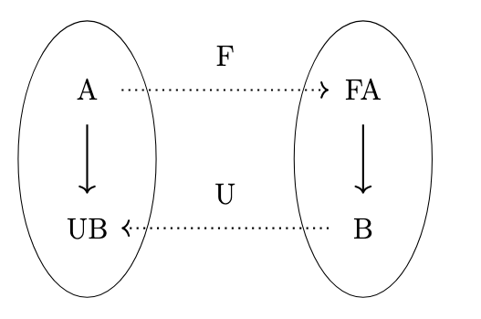
In other words, \(\mathrm{Hom}_{\mathbf{Mon}}(FA,B) \cong \mathrm{Hom}_{\mathbf{Set}}(A,UB)\). If let \(U\) be the so-called _forgetful functor_ which maps each monoid to its underlying set and each monoid homomorphism to its underlying function and \(F\) be the functor that maps each set \(A\) to its corresponding monoid \((A*,+,\epsilon_A)\) and each functor \(f\) to the function \(Ff\) such that \(Ff([a_1,a_2,\dots,a_n]) = [f(a_1),f(a_2),\dots,f(a_n)]\), then we have a pair of adjoint functors.
Naturality
Let \(\phi : \mathrm{Hom}_{\mathbf{Mon}}(FA,B) \rightarrow \mathrm{Hom}_{\mathbf{Set}}(A,UB)\) be the mapping \(\phi(h)(a) = h([a])\) and \(\phi^{-1} : \mathrm{Hom}_{\mathbf{Set}}(A,UB) \rightarrow \mathrm{Hom}_{\mathbf{Mon}}(FA,B)\) be the mapping \(\phi^{-1}(f)([a_1,a_2,\dots,a_n]]) = f(a_1)+f(a_2)+...+f(a_n)\). The following diagrams commute.
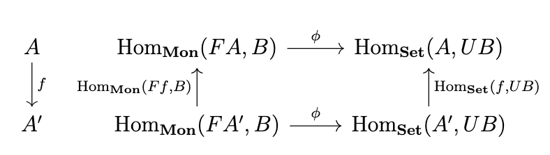
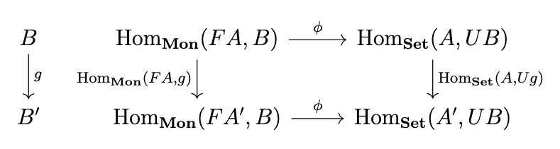
Note that for any \(h \in \mathrm{Hom}_{\mathbf{Mon}}(FA',B)\) and \(a \in A\), the following equation holds.
\begin{split}(\phi \circ \mathrm{Hom}_{\mathbf{Mon}}(Ff,B))(h)(a) & = \phi(\mathrm{Hom}_{\mathbf{Mon}}(Ff,B)(h))(a) \\& = \phi(h \circ Ff)(a) \\& = h(Ff([a])) \\& = h([f(a)]) \\& = \phi(h)(f(a)) \\& = (\phi(h) \circ f)(a) \\& = \mathrm{Hom}_{\mathbf{Set}}(f,B)(\phi(h))(a) \\& = (\mathrm{Hom}_{\mathbf{Set}}(f,B) \circ \phi)(h)(a).\end{split}
Note that for any \(h \in \mathrm{Hom}_{\mathbf{Mon}}(FA,B)\) and \(a \in A\), the following equation holds.
\begin{split}(\phi \circ \mathrm{Hom}_{\mathbf{Mon}}(FA,g))(h)(a) & = \phi(\mathrm{Hom}_{\mathbf{Mon}}(FA,g)(h))(a) \\& = \phi(g \circ h)(a) \\& = (g \circ h)([a]) \\& = g(h([a])) \\& = Ug(h([a])) \\& = Ug(\phi(h)(a)) \\& = (Ug \circ \phi(h))(a) \\& = \mathrm{Hom}_{\mathbf{Set}}(A,Ug)(\phi(h))(a) \\& = (\mathrm{Hom}_{\mathbf{Set}}(A,Ug) \circ \phi)(h)(a)\end{split}
Unit
Let us consider what the unit of this adjunction must be. The unit \(\eta : 1 \rightarrow UF\) is a natural transformation such that for any \(f : A \rightarrow UB\) there exists a unique monoid homomorphism \(h : FA \rightarrow B\) such that the following diagram commutes.
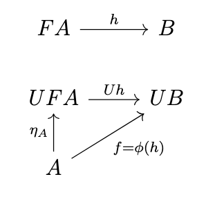
In fact, this is the usual definition of a free monoid (i.e. in terms of the universal property of the unit). This means that \(Uh \circ \eta_A = \phi(h)\) and thus for any \(a \in A\), the following equivalences hold.
\begin{split}(Uh \circ \eta_A)(a) & = \phi(h)(a) \\& = h([a]) \\& = Uh([a])\end{split}
Thus, we have that \(Uh(\eta_A(a)) = Uh([a])\). Now, since the above diagram must commute for any \(f = \phi(h)\), then it must commute for injective \(f\); if \(f\) is injective, then so is \(h\), and thus the equation \(Uh(\eta_A(a)) = Uh([a])\) implies that \(\eta_A(a) = [a]\). Thus, the only way to guarantee that the unit suffices for arbitrary \(f\) is to set \(\eta_A(a) = [a]\). Thus, the unit maps each element to its corresponding singleton list.
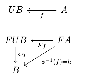
Counit
Next, let us consider the counit of this adjunction. The counit \(\epsilon : FU \rightarrow 1\) is a natural transformation such that for any \(h : FA \rightarrow B\) there exists a unique function \(f : A \rightarrow UB\) such that the following diagram commutes.
As we established previously, the adjunction \((F,U,\eta,\epsilon)\) induces a monad \((T=UF,\mu=U\epsilon_F,\eta)\). Let us consider what \(\mu = U\epsilon_F\) must represent; substituting \(FB\) for \(B\) and applying \(U\), we obtain the following diagram.
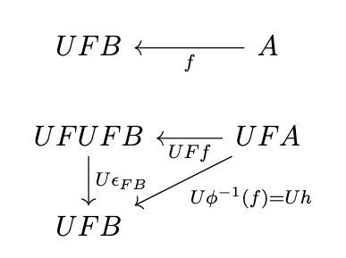
Thus, \(U\epsilon_{FB} \circ UFf = U\phi^{-1}(f)\). We have the simplifications in the following equations.
\begin{split}(U\epsilon_{FB} \circ UFf)([a_1,a_2,...,a_n]) & = U\epsilon_{FB}(UFf([a_1,a_2,\dots,a_n])) \\& = U\epsilon_{FB}(Ff([a_1,a_2,\dots,a_n])) \\& = U\epsilon_{FB}([f(a_1),f(a_2),\dots,f(a_n)]) \\\end{split}
\begin{split}U\phi^{-1}(f)([a_1,a_2,\dots,a_n]) & = \phi^{-1}(f)([a_1,a_2,\dots,a_n]) \\& = f(a_1) + f(a_2) + \dots + f(a_n)\end{split}
Thus, we have determined that \(U\epsilon_{FB}([f(a_1),f(a_2),\dots,f(a_n)]) = f(a_1) + f(a_2) + \dots + f(a_n)\). Since each \(f(a_i)\) is a list, \(\mu\) therefore joins a list of lists of elements into a corresponding list of elements.
Lists in the Semantic Category
Now that we have analyzed the situation in \(\mathbf{Set}\), we can drop our tentative definition of the free monoid on a set \(A\) as \((A^*,+,\epsilon)\), define the functor \(F\) to be the left adjoint to the functor \(U\), and _define_ the free monoid on a set \(A\) to be \(FA\). Thus, \((A^*,+,\epsilon)\) is simply a canonical example of a free monoid on \(A\); anything isomorphic to it also qualifies. Additionally, this definition has the advantage that it can be applied to other categories besides \(\mathbf{Set}\). Thus, we assume that the semantic category \(\mathcal{C}\) for a programming language has a list type and a monoid type. We can define a subcategory \(\mathbf{Mon}_{\mathcal{C}}\) of monoids in \(\mathcal{C}\), as depicted in the following figure.
We summarize the list monad translations in the following table.
| Monad Component | Lambda Term |
|---|---|
| \(Tf\) | \(\lambda [a_1, a_2, \dots, a_n] . [f a_1, f a _2,\dots, f a_n]\) |
| \(\eta_A\) | \(\lambda a . [a]\) |
| \(\mu_A\) | \(\lambda [l_1, l_2, \dots, l_n] . l_1 + l_2 + \dots + l_n\) |
| \(f^*\) | \(\lambda [a_1, a_2, \dots, a_n] . f a_1 + f a_2 + \dots + f a_n\) |
The State Monad
The state monad represents computations that read or update an external environment (i.e. functions with side effects that update memory state). We model a computation \(A \rightarrow B\) between types \(A\) and \(B\) that updates an environment of type \(E\) by a morphism \(A \times E \rightarrow B \times E\). We may think of this as a pair of morphisms, one that performs the basic computation, and one that updates the state of the environment.
More generally, we can model this situation in a monoidal category \((\mathcal{C},\otimes)\) which is thus equipped with a tensor product; the computation is then modeled as a morphism \(A \otimes E \rightarrow B \otimes E\).
Internal Hom
Computer scientists and programmers will be familiar with the notion of currying, i.e., that each function of the form \(\lambda \langle a,b \rangle.f(a,b)\) is equivalent to a function of the form \(\lambda a . \lambda b . f(a,b)\) and vice versa. We can represent a function that takes two arguments such as \(\lambda \langle a,b \rangle.f(a,b)\) as a type \(A \otimes B \rightarrow C\) and we can represent a curried function such as \(\lambda a . \lambda b . f(a,b)\) as a type \(A \rightarrow [B,C]\), where \([B,C]\) denotes an _internal hom object_, i.e. an object that represents all morphisms \(B \rightarrow C\). It is an internal abstraction of the external hom set \(\mathrm{Hom}_{\mathcal{C}}(B,C)\). Thus, we have the situation depicted in the following figure.
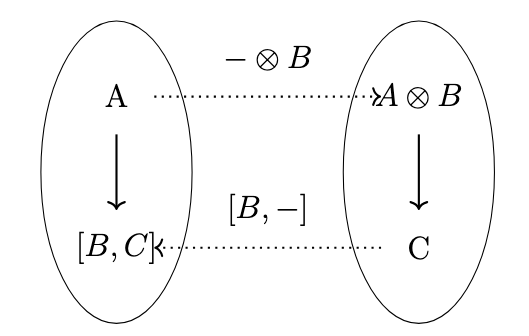
Thus, we have that \(\mathrm{Hom}_{\mathcal{C}}(A \otimes B, C) \cong \mathrm{Hom}_{\mathcal{C}}(A,[B,C])\). We intend, moreover, that this correspondence be natural in \(A\) and \(C\), that is, that the functor \(- \otimes B\) be left-adjoint to the functor \([B,-]\). Since we are given the functor \(- \otimes B\) in a monoidal category, we can define the internal hom functor \([B,-]\) as the right adjoint to \(- \otimes B\).
Thus, we have a pair of adjoint functors, one for each object \(B\). We may think of the functors \([B,-]\) as a family of functors \(U_B = [B,-]\) _indexed_ by the object \(B\) of the category \(\mathcal{C}\). We will later establish that \([-,-]\) comprises a bifunctor, in which case we may also think of the functors \([B,-]\) as parameterized adjoints.
Recovering the External Hom
In any monoidal category, \(B \otimes I \cong B \cong I \otimes B\) for any object \(B\), where \(I\) is the designated unit object. Thus, the following diagram commutes.
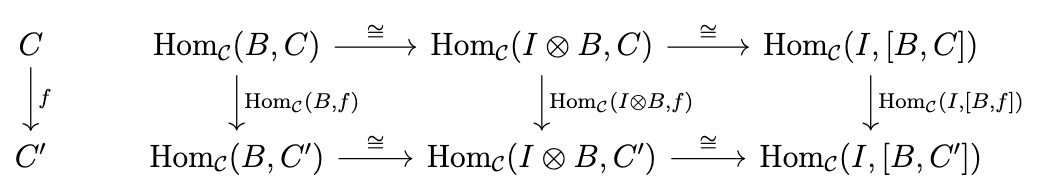
In other words, \(\mathrm{Hom}_{\mathcal{C}}(B,C) \cong \mathrm{Hom}_{\mathcal{C}}(I,[B,C])\) and \(\mathrm{Hom}_{\mathcal{C}}(B,f) \cong \mathrm{Hom}_{\mathcal{C}}(I,[B,f])\) for all objects \(B\) and \(C\) and morphisms \(f : C \rightarrow C'\) of \(\mathcal{C}\); that is, for "locally-small" categories (categories with an external hom-set), we can recover the external hom-set and the hom-functor from the internal hom
Defining \([-,C]\)
We want to be able to define the functor \([-,C] : \mathcal{C}^{op} \rightarrow \mathcal{C}\) for all objects \(C\) of \(\mathcal{C}\) as well. In order for the isomorphism \(\mathrm{Hom}_{\mathcal{C}}(A \otimes -, C) \cong \mathrm{Hom}_{\mathcal{C}}(A,[-,C])\) to hold, the functor \([-,C]\), the functor \([-,C]\) must be contravariant, in order that the variance of both sides of this isomorphism are consistent. This is in accordance with the analogy to \(\mathrm{Hom}_{\mathcal{C}}(-,C)\), which is contravariant.
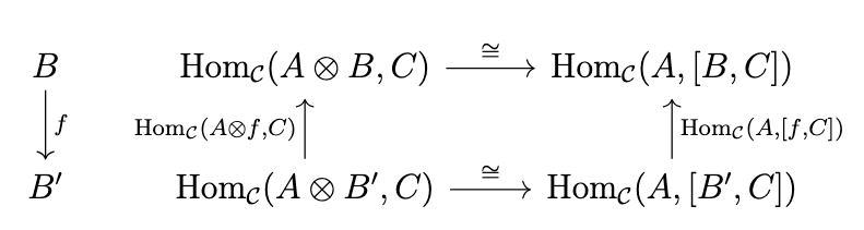
We further desire that the isomorphism \(\mathrm{Hom}_{\mathcal{C}}(A \otimes B, C) \cong \mathrm{Hom}_{\mathcal{C}}(A,[B,C])\) be natural in \(B\). This means that the following diagram commutes.
Letting \(U = [B,-]\), \(U' = [B',-]\), \(F = - \otimes B\), \(F' = - \otimes B'\), \(\sigma = - \otimes f\), and \(\tau = [f,-]\), we abstract the previous diagram as the following diagram.
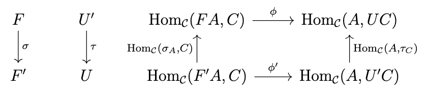
Thus, we have two adjunctions \(\langle F,U,\phi,\eta,\epsilon \rangle\) and \(\langle F',U',\phi',\eta',\epsilon' \rangle\), and morphisms \(\sigma : F \rightarrow F'\) and \(\tau : U' \rightarrow U\) between their respective functors that preserve their respective isomorphisms, i.e., we have a suitable notion of a transformation of adjoints. We call such a pair of natural transformations \(\langle \sigma, \tau \rangle\) that makes the above diagram commute a conjugate pair.
Determining Conjugate Pairs
Now, given \(\sigma\), we want to determine \(\tau\). We chase the identity \(1_{U'C} \in \mathrm{Hom}_{\mathcal{C}}(U'C,U'C)\) around the following diagram
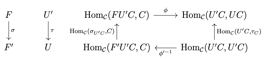
in order to compute a morphism equivalent to \(\tau_C\) as shown in the following diagram.
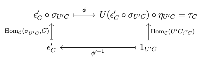
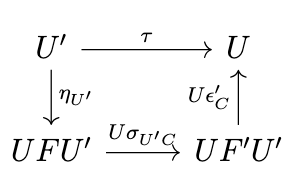
Thus, we have determined that the following diagram commutes.

In fact, the converse is true: the equation in the previous diagram is sufficient to ensure that \(\langle \sigma, \tau \rangle\) is a conjugate pair, since for any \(g : A \rightarrow U'C \in \mathrm{Hom}_{\mathcal{C}}(A,U'C)\), the following equation holds.
\begin{split}(\phi \circ \mathrm{Hom}_{\mathcal{C}}(\sigma_A,C) \circ \phi'^{-1})(g) & = (\phi \circ \mathrm{Hom}_{\mathcal{C}}(\sigma_A,C))(\epsilon'_C \circ F'g) \\& = \phi(\epsilon'_C \circ F'g \circ \sigma_A) \\& = U(\epsilon'_C \circ F'g \circ \sigma_A) \circ \eta_A \\& = U\epsilon'_C \circ UF'g \circ U\sigma_A \circ \eta_A \\& = U\epsilon'_C \circ U\sigma_{U'C} \circ UFg \circ \eta_A \\& = U\epsilon'_C \circ U\sigma_{U'C} \circ \eta_{U'C} \circ g \\& = \tau_C \circ g \\& = \mathrm{Hom}_{\mathcal{C}}(A,\tau_C)(g)\end{split}
The third and fourth to the last equations in the previous derivation are by the naturality of \(\sigma\) and \(\eta\), respectively.
Thus, \(\langle \sigma, \tau \rangle\) is a conjugate pair if and only if \(\tau = U\epsilon' \circ U\sigma_{U'} \circ \eta_{U'}\). Since \(\tau\) is determined by an equation, it is also unique.
Definition of \([-,C]\)
We can now determine by the following diagram that \([f,C] = [B, \epsilon'_C \circ [B',C] \otimes f] \circ \eta_{[B'C]}\).
We intend for the morphism \([f,C]\) to be analogous to the function \(\mathrm{Hom}_{\mathcal{C}}(f,C)\), i.e., the mapping \(g \mapsto g \circ f\) for \(g: B' \rightarrow C\), as shown in the following diagram.
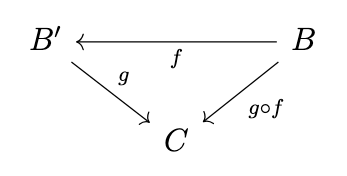
Translating to the Lambda Calculus
In the lambda calculus, the composition \(g \circ f\) is represented as a term \(\lambda b . g (f b)\). The mapping \(g \mapsto g \circ f\) is then represented as a term \(\lambda g . \lambda b . g (f b)\), which has the "uncurried" form \(\lambda \langle g, b \rangle . g (f b)\).
The component \(\epsilon'_C : [B',C] \otimes B' \rightarrow C\) of the counit corresponds to the term \(\lambda \langle g, b' \rangle . gb'\) which intuitively represents an evaluation function, i.e., a function which takes a pair consisting of a function and a value and applies the function to the value.
The morphism \([B',C] \otimes f : [B',C] \otimes B \rightarrow [B',C] \otimes B'\) corresponds to the term \(\lambda \langle g, b \rangle . \langle g, f b \rangle\).
Thus, composing these terms yields the term \(\lambda \langle g, b \rangle . (\lambda \langle \overline{g}, b' \rangle . \overline{g} b')(\lambda \langle \overline{\overline{g}},\overline{b} \rangle . \langle \overline{\overline{g}},f\overline{b} \rangle)\langle g,b\rangle\), which simplifies to \(\lambda \langle g, b \rangle . g (f b)\).
The term \(\lambda \langle g, b \rangle . g (f b)\) thus corresponds to the following diagram, which intuitively applies \(f\) to \(b\) and then evaluates \(g (f b)\), as shown in the following diagram.
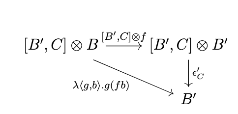
Finally, we curry \(\lambda \langle g, b \rangle . g (f b)\) to obtain \(\lambda g . \lambda b . g (f b)\) which corresponds to \(\phi(\epsilon'_C \circ [B',C] \otimes f) = [B, \epsilon'_C \circ [B',C] \otimes f] \circ \eta_{[B'C]}\). Thus, the morphism \([f,C]\) has precisely the interpretation that we expect.
We have thus established a sort of dictionary for translating between various elements of our categorical model and terms of the lambda calculus, as shown in the following table.
| Mathematical Expression | Lambda Term |
|---|---|
| \([X,Y]\) | functions of the form \(\lambda x . y\) |
| \(X \otimes Y\) | pairs of the form \(\langle x,y\rangle\) |
| \(A \otimes f : A \otimes X \rightarrow A \otimes Y\) | \(\lambda \langle a,x\rangle . \langle a,f x\rangle\) |
| \(f \otimes A : X \otimes A \rightarrow Y \otimes A\) | \(\lambda \langle x,a\rangle . \langle f x,a\rangle\) |
| \(g \circ f\) | \(\lambda x . g (f x)\) |
| \(\epsilon_X\) | \(\lambda \langle f,x\rangle . f x\) |
| \([X,f]\) | \(\lambda g . \lambda x . f (g x)\) |
| \([f,X]\) | \(\lambda g . \lambda x . g (f x)\) |
The Induced Monad
We now determine what the induced monad \((T,\mu,\eta)\) must represent. Here we assume a fixed "environment" type of \(B\).
For the functor \(T = [B, - \otimes B]\), \(TA = [B, A \otimes B]\) and \(T(f : A \rightarrow A') = [B,f \otimes B] : [B, A \otimes B] \rightarrow [B, A' \otimes B]\). Using our dictionary, \([B, f \otimes B]\) corresponds to a term \(\lambda g . \lambda b . h (g b)\) where \(h = \lambda \langle a,b\rangle . \langle fa,b\rangle\) represents \(f \otimes B\).
Each component \(\mu_A = [B, \epsilon_{A \otimes B}] : [B,[B,A \otimes B] \otimes B] \rightarrow [B, A \otimes B]\) corresponds to a term \(\lambda g . \lambda b . \epsilon_{A \otimes B} (g b)\) which in turn corresponds to the term \(\lambda g . \lambda b . (\lambda \langle f,\langle a,\overline{b}\rangle\rangle . f \langle a,\overline{b}\rangle) (g b)\).
Each component \(\eta_A : A \rightarrow [B,A \otimes B]\) is equal to \(\phi(1_{A \otimes B})\), and hence is the curried form of the identity function \(\lambda \langle a,b\rangle . \langle a,b\rangle\), that is the function \(\lambda a . \lambda b . \langle a,b\rangle\).
Next, we consider what the Kleisli lifting \(f^* = \mu_B \circ Tf\) for \(f : A \rightarrow B\) must be. The lifting \(\mu_B \circ Tf\) corresponds to (\ref{state-monad-kleisli-lifting}) by our dictionary, which simplifies to \(\lambda \overline{\overline{g}} . \lambda b . (\lambda \langle f,p \rangle . f p)((\lambda \langle a,\overline{\overline{b}} \rangle . \langle f a, \overline{\overline{b}}\rangle)(\overline{\overline{g}} b))\). Thus, we have obtained the translations summarized as follows.
\[\(\lambda \overline{\overline{g}} . (\lambda g . \lambda b . (\lambda \langle f,p\rangle . f p)(g b))((\lambda \overline{g} . \lambda \overline{b} . (\lambda \langle a,\overline{\overline{b}}\rangle . \langle f a,\overline{\overline{b}}\rangle)(\overline{g} \overline{b})) \overline{\overline{g}})\]
| Monad Component | Lambda Term |
|---|---|
| \(Tf\) | \(\lambda g . \lambda b . (\lambda \langle a,\overline{b}\rangle . \langle f a, \overline{b}\rangle)(g b)\) |
| \(\eta_A\) | \(\lambda a . \lambda b . \langle a,b\rangle\) |
| \(\mu_A\) | \(\lambda g . \lambda b . (\lambda \langle f,p\rangle . f p)(g b)\) |
| \(f^*\) | \(\lambda g . \lambda b . (\lambda \langle f,p \rangle . f p)((\lambda \langle a,\overline{b} \rangle . \langle f a, \overline{b}\rangle)(g b))\) |
The Continuation Monad
The continuation monad represents computations in continuation-passing style. A function \(\lambda x . y\) corresponds to a continuation-passing style function \(\lambda x . \lambda k . k y\), i.e. an augmented function which additionally accepts a continuation function \(k\) and "continues" by evaluating \(k\) with parameter \(y\) rather than "returning" (i.e. evaluating to \(y\)).
We model a continuation-passing style function \(\lambda x . \lambda k . k y\) as a morphism \(X \rightarrow [[Y, Z],Z]\). We want a morphism \(X \rightarrow Y\) in the Kleisli category \(\mathcal{C}_T\) to correspond to a morphism \(X \rightarrow [[Y, Z],Z]\) in the category of types \(\mathcal{C}\). Thus, we choose the underlying functor of the continuation monad to be \(T = [[-,Z],Z]\) so that a morphism \(X \rightarrow TY\) corresponds to \(X \rightarrow [[Y, Z],Z]\). There is one such \(T\) per choice of object \(Z\).
Self-Dual Adjunction of \([-,Z]\)
Recall that a contravariant functor such as \([-,Z]\) can be considered a functor \([-,Z] : \mathcal{C}^{op} \rightarrow \mathcal{C}\) or a functor \([-,Z]^* : \mathcal{C} \rightarrow \mathcal{C}^{op}\). Thus, we can view the functor \([[-,Z],Z] : \mathcal{C} \rightarrow \mathcal{C}\) as the composition indicated in the following diagram.
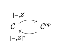
Note the situation depicted in the following figure.
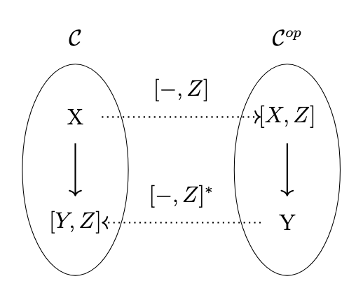
By the hom-tensor adjunction, and since we are assuming that \(\mathcal{C}\) is symmetric monoidal, we have the following equivalences.
\begin{split}\mathrm{Hom}_{\mathcal{C}}(X,[Y,Z]) & \cong \mathrm{Hom}_{\mathcal{C}}(X \otimes Y,Z) \\& \cong \mathrm{Hom}_{\mathcal{C}}(Y \otimes X,Z) \\& \cong \mathrm{Hom}_{\mathcal{C}}(Y,[X,Z]) \\& \cong \mathrm{Hom}_{\mathcal{C}^{op}}([X,Z],Y) \\\end{split}
Thus, since these isomorphisms are natural, \([-,Z]\) is a "self-dual" adjoint.
The Induced Monad
Intuitively, the isomorphism \(\mathrm{Hom}_{\mathcal{C}}(X,[Y,Z]) \cong \mathrm{Hom}_{\mathcal{C}^{op}}([X,Z],Y)\) indicates that each function of the form \(\lambda x . \lambda y . z\) is equivalent to a function of the form \(\lambda y . \lambda x . z\), i.e. one with the "arguments" reversed.
Since the functor \([-,Z]\) is "self-dual", the unit and counit of the adjunction coincide. For \(f : [X,Z] \rightarrow Y\) in \(\mathcal{C}^{op}\) (which corresponds to a morphism \(f : Y \rightarrow [X,Z]\) in \(\mathcal{C}\)) and \(\phi : \mathrm{Hom}_{\mathcal{C}^{op}}([X,Z],Y) \rightarrow \mathrm{Hom}_{\mathcal{C}}(X,[Y,Z])\), the unit diagram is indicated in the following diagram.
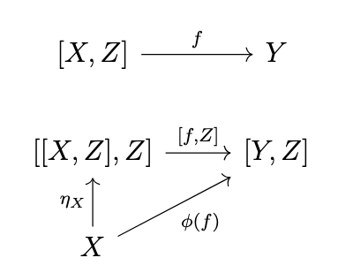
The component \(\eta_X\) then corresponds to a term \(\lambda x . \lambda k . k x\). To confirm this, note that \([f,Z] \circ \eta_X\) then corresponds by our prior dictionary to the term \(\lambda x . (\lambda g . \lambda y . g (f y))((\lambda \overline{x} . \lambda k . k \overline{x}) \overline{x})\). The morphism \(f\) then corresponds to a term \(\lambda y . \lambda x . z(x,y)\), where \(z(x,y)\) explicitly indicates the dependence of the term \(z\) on \(x\) and \(y\). We then have the following equivalences.
\begin{split}\lambda x . (\lambda g . \lambda y . g (f y))((\lambda \overline{x} . \lambda k . k \overline{x}) x) & = \lambda x . (\lambda g . \lambda y . g (f y)) (\lambda k . k x) \\& = \lambda x . \lambda y (\lambda k . k x)(f y) \\& = \lambda x . \lambda y (\lambda k . k x)((\lambda \overline{y} . \lambda \overline{x} . z(\overline{x},\overline{y})) y) \\& = \lambda x . \lambda y . (\lambda k . k x) (\lambda \overline{x} . z(\overline{x},y)) \\& = \lambda x . \lambda y . z(x,y)\end{split}
Thus, this is indeed equivalent to the term \(\lambda x . \lambda y . z(x,y)\) which corresponds to the morphism \(\phi(f)\).
The functor \(T = [[-,Z],Z]\) applied to a morphism \(f : X \rightarrow X'\) yields a morphism \([[f,Z],Z] : [[X,Z],Z] \rightarrow [[X',Z],Z]\); the morphism \([f,Z]\) corresponds by our prior dictionary to the term \(\lambda g . \lambda x . g (f x)\) and the morphism \([[f,Z],Z]\) in turn corresponds to the term \(\lambda \overline{g} . \lambda k . \overline{g} ((\lambda g . \lambda x . g (f x)) k)\), which simplifies to \(\lambda \overline{g} . \lambda k . \overline{g}(\lambda x . k (f x))\).
The natural transformation \(\mu = [\eta_{[-,Z]},Z]\) has component \(\mu_X = [\eta_{[X,Z]},Z]\); letting the term \(\lambda g . \lambda k . k g\) represent \(\eta_{[X,Z]}\), the term \(\lambda \overline{g} . \lambda h . \overline{g} ((\lambda g . \lambda k . k g) h)\) then corresponds to \([\eta_{[X,Z]},Z]\). This simplifies to \(\lambda \overline{g} . \lambda h . \overline{g}(\lambda k . k h)\).
The Kleisli lifting \(\_^*\) is defined such that \(f^* = \mu_B \circ Tf\) for \(f : A \rightarrow TB\). By our dictionary, \(\mu_B \circ Tf\) corresponds to the term \(\lambda g (\lambda \overline{g} . \lambda h . \lambda \overline{g} (\lambda k . k h))((\lambda \overline{\overline{g}} . \lambda \overline{k} . \overline{\overline{g}}(\lambda x . k (f x)))g)\). This simplifies to \(\lambda g . \lambda h . g (\lambda x . (f x) h)\).
Thus, we've obtained the translations summarized in the following table.
| Monad Component | Lambda Term |
|---|---|
| \(Tf\) | \(\lambda g . \lambda k . g(\lambda x . k (f x))\) |
| \(\eta_X\) | \(\lambda x . \lambda k . k x\) |
| \(\mu_X\) | \(\lambda g . \lambda h . g(\lambda k . k h)\) |
| \(f^*\) | \(\lambda g . \lambda h . g (\lambda x . (f x) h)\) |
The Haskell Monad Typeclass
In Haskell, the Monad typeclass is defined in the following listing. We omit miscellaneous functions from various typeclasses where they are not relevant.
class Applicative m => Monad m where
    (>>=)  :: m a -> (a -> m b) -> m b
    return :: a -> m a
Presentation as Kleisli Triple
In Haskell, the Monad typeclass is presented as a Kleisli triple \((T,\eta,\_^*)\). The functor \(T\) is implemented via the fmap function of the Functor typeclass, which Monad extends, as shown in the following listing.
class Functor f where
    fmap :: (a -> b) -> f a -> f b
Just as \(T(f : A \rightarrow B) : TA \rightarrow TB\), so also `fmap f :: fa -> fb}. Every Functor instance is required to satisfy the laws specified in the following listing.
fmap id  ==  id
fmap (g . f)  ==  fmap g . map f
These laws clearly correspond to the requirements for a functor \(T\), i.e., that \(T(1_A) = 1_{TA}\) and \(T(g \circ f) = Tg \circ Tf\).
The mapping \(\eta\) of a Kleisli triple corresponds to the function return :: a -> m a of the Monad typeclass.
The function >>= (pronounced "bind") represents the lifting (\(\_^*\)) of the Kleisli triple. A morphism \(f : A \rightarrow TB\) corresponds to a function f :: a -> m b, and the extension \(f^* : TA \rightarrow TB\) corresponds to (>>= f) :: ma -> mb.
Thus, since Kleisli composition is defined as \(g^* \circ f\), we can define Kleisli composition (denoted >=>, the "Kleisli fish" in Haskell) as indicated in the following listing.
(>=>) :: Monad m => (a -> mb) -> (b -> mc) -> (a -> mc)
f >=> g = (>>= g) . f
Indeed, this is precisely how Kleisli composition is defined in the Control.Monad module, shown as follows.
(>=>) :: Monad m => (a -> mb) -> (b -> mc) -> (a -> mc)
f >=> g = \x -> f x >>= g
Note, however, that our definition uses the so-called "point-free" style, i.e. it uses composition instead of application, eliminating the unnecessary function argument (i.e., "point").
Monad Laws
Every Monad instance is required to satisfy the three laws stated as follows.
m >>= return  ==  m
return a >>= k  ==  k a
m >>= (x -> k x >>= h)  ==  (m >>= k) >>= h
The Monad laws correspond precisely to the axioms of a Kleisli triple, as indicated in the following table.
| Haskell Monad Law | Kleisli Triple Axiom |
|---|---|
m >>= return == m |
\(\eta_A^* = 1_{TA}\) |
return a >>= k == k a |
\(f^* \circ \eta_A = f\) |
m >>= (\textbackslash x -> k x >>= h) == (m >>= k) >>= h |
\((g^* \circ f)^* = g^* \circ f^*\) |
Point-Free Monad Laws
The correspondence in the previous table is somewhat opaque, due to the use of "pointed" functions, so we rewrite the Monad laws to use point-free style. Note the transformations in the following listings.
-- original law:
m >>= return == m
-- prefix instead of infix:
(>>= return) m == m
-- definition of id:
(>>= return) m == id m
-- function equivalence:
(>>= return) = id
-- original law:
return a >>= k == k a
-- prefix instead of infix:
(>>= k) (return a) == k a
-- definition of composition:
((>>= k) . return) a == k a
-- function equivalence:
(>>= k) . return == k-- original law:
m >>= (\x -> k x >>= h) == (m >>= k) >>= h
-- prefix instead of infix:
m >>= (\x -> (>>= h)(k x)) == (m >>= k) >>= h
-- definition of composition:
m >>= (\x -> ((>>= h) . k) x) == (m >>= k) >>= h
-- lambda abstraction:
m >>= ((>>= h) . k) == (m >>= k) >>= h
-- prefix versus infix:
(>>= ((>>= h) . k) m == (m >>= k) >>= h
-- prefix versus infix:
(>>= ((>>= h) . k) m == (>>= h) (m >>= k)
-- prefix versus infix:
(>>= ((>>= h) . k) m == (>>= h) ((>>= k) m)
-- definition of composition:
(>>= ((>>= h) . k) m == ((>>= h) . (>>= k)) m
-- function equivalence:
(>>= ((>>= h) . k) == ((>>= h) . (>>= k))Thus, renaming the various functions, we have the following equivalent laws for a Monad in Haskell.
(>>= return)  ==  id
(>>= f) . return  ==  f
(>>= ((>>= g) . f)) == (>>= g) . (>>= f)
Using the translation of (>>= f) to \(f^*\) and return to \(\eta_A\), it is now easy to see how these laws correspond to the axioms of a Kleisli triple exactly, as indicated in the following table.
| Point-Free Haskell Monad Law | Kleisli Triple Axiom |
|---|---|
(>>= return) == id |
\(\eta_A^* = 1_{TA}\) |
(>>= f) . return == f |
\(f^* \circ \eta_A = f\) |
(>>= ((>>= g) . f)) == (>>= g) . (>>= f) |
\((g^* \circ f)^* = g^* \circ f^*\) |
Direct Monad Presentation
Haskell also defines a join :: Monad m => m (m a) -> m a function which represents the natural transformation \(\mu : T^2 \rightarrow T\) of the respective monad. As we previously determined, we can define \(\mu_A = 1_{TA}^*\). Thus, translating this into Haskell, we obtain the following function.
join :: Monad m => m (m a) -> m a
join = (>>= id)
Indeed, this is precisely how this function is defined in the Control.Monad module, except that our definition is point-free, as shown in the following listing.
join :: Monad m => m (m a) -> m a
join x = x >>= id
In the Haskell Control.Monad module, there is a naming convention that functions suffixed with "M" are related to morphisms in the Kleisli category of a monad (which correspond to morphisms \(A \rightarrow TB\)), e.g. filterM, as shown in the following listing.
filter :: (a ->   Bool) -> [a] ->   [a]
filterM :: Monad m => (a -> m Bool) -> [a] -> m [a]
We could alternatively define the Monad typeclass using join and return, which corresponds directly to the mathematical concept, as indicated in the following listing.
class Functor m => Monad m where
    join :: m (m a) -> m a
    return :: a -> m a
The Monad Laws
Given the previous presentation, the monad laws would then be as indicated in the following table.
| Haskell Monad Law | Monad Equation |
|---|---|
join . (fmap . fmap) f == fmap f . join |
\(\mu_B \circ T^2f = Tf \circ \mu_A\) (naturality of \(\mu\)) |
return . f == fmap f . return |
\(\eta_B \circ f = Tf \circ \eta_A\) (naturality of \(\eta\)) |
join . fmap join == join . join |
\(\mu \circ T\mu = \mu \circ \mu_T\) (associativity of \(\mu\)) |
join . fmap return == id |
\(\mu \circ T\eta = 1_T\) (left unitality of \(\eta\)) |
join . return == id |
\(\mu \circ \eta_T = 1_T\) (right unitality of \(\eta\)) |
Then, we could redefine >>= and >>=> as indicated in the following listing.
(>>=) :: Monad m => m a -> (a -> m b) -> m b
m >>= f = (join . fmap f) m


(>=>) :: Monad m => (a -> m a) -> (b -> m c) -> (a -> m c)
f >=> g = join . fmap g . f
Java Monads
Monads are implicit in Java 8 in the Stream interface and Optional class. There is no explicit Monad interface because it is impossible to define such an interface due to Java's lack of higher-order polymorphism. In other words, we cannot write the interface defined in the following pseudocode listing.
public interface (Functor F)<A> {
    <B> F<B> map (Function<? super A, B> f);
}
Although we cannot correctly define an abstract Monad interface in Java, we can nonetheless define individual concrete instances of monads. For instance, JDK 8 defines the Optional class as indicated in the following listing, where we omit irrelevant methods.
public final class Optional<T> {
    public <U> Optional<U> map(Function<? super T,? extends U> mapper);
    public static <T> Optional<T> of(T value);
    public <U> Optional<U> flatMap(Function<? super T,Optional<U>> mapper);
}
Since Java functions are methods of classes, each method is implicitly invoked with a parameter representing the instance of the object upon which the method was invoked (i.e., the this reference). Thus, rewriting the method signatures of the Optional class to be static, we obtain the following listing.
    public static <T, U> Optional<U> map(Function<? super T,? extends U> mapper, Optional<T> instance);
    public static <T> Optional<T> of(T value);
    public static <T, U> Optional<U> flatMap(Function<? super T,Optional<U>> mapper, Optional<T> instance);
In this form it is clear that map corresponds to Haskell's fmap, of corresponds to Haskell's return, and flatMap corresponds to Haskell's >>=.
Implementing Monads
We now give examples of implementations for each of the monads discussed above. Each monad is presented as a Kleisli triple, as described previously.
Note, however, that these implementations are pared down to the essentials. In Haskell, we do not consider issues of strict versus non-strict evaluation, and in Java we do not consider null checks and laziness, etc.
In Haskell, we define our own Monad and Functor typeclasses, hiding those defined in the prelude for the sake of simplicity, as shown in the next listing. Implementing the additional functions of those interfaces is straightforward.
import Prelude hiding (Monad, (>>=), return, Functor, fmap)
class Functor f where
    fmap :: (a -> b) -> f a -> f b


class Functor m => Monad m where
    return :: a -> m a
    (>>=) :: m a -> (a -> m b) -> m b
The Identity Monad
We begin with the identity monad.
Haskell
In Haskell, we represent the identity monad with a type, Identity, as shown in the following listing.
newtype Identity a = Identity { runIdentity :: a }

instance Functor Identity where
    fmap f = Identity . f . runIdentity


instance Monad Identity where
    return = Identity
    m >>= k = k $ runIdentity m
This type has a single unary type constructor Identity :: a -> Identity a. We declare the Identity type with a newtype declaration, which indicates that the types a and Identity a are considered isomorphic, i.e., the equivalences in the following listing hold. It is in this sense that it is an "identity". The Identity a type can be viewed as a sort of synonym for the type a.
runIdentity . Identity == id
Identity . runIdentity == id
Java
We likewise represent the identity monad in Java with a type Identity<T>, as shown in the following listing.
import java.util.function.Function;

public class Identity<T> {
    private final T value;

    public Identity(final T value) {
        this.value = value;
    }

    public static <V> Identity<V> of(final V value) {
        return new Identity<>(value);
    }

    public <V> Identity<V> map(final Function<? super T, V> f) {
        return new Identity<>(f.apply(this.value));
    }

    public <V> Identity<V> flatMap(final Function<? super T, Identity<V>> k) {
        return k.apply(this.value);
    }
}
The Maybe Monad
Next, we describe the maybe monad.
Haskell
In Haskell, coproducts are represented with sum types. The coproduct \(A + 1\) is represented by the sum type Maybe a which has two type constructors, a unary type constructor Just which "tags" results of computations, and a nullary type constructor Nothing which represents the "bottom" value \(\bot\), as shown in the following listing.
data Maybe a = Just a | Nothing

instance Functor Maybe where
    fmap f (Just a) = Just $ f a
    fmap f Nothing = Nothing

instance Monad Maybe where
    return = Just
    (Just a) >>= k = k a
    Nothing >>= _ = Nothing
Java
Java lacks sum types. Thus, we use a special, designated singleton instance NOTHING object to represent the "bottom" value, as shown in the following listing.
import java.util.function.Function;

public class Maybe<T> {

    private static final Maybe<?> NOTHING = new Maybe<>();

    private final T value;

    public Maybe(final T value) {
        this.value = value;
    }

    private Maybe() {
        this.value = null;
    }

    public static <V> Maybe<V> of(final V value) {
        return new Maybe<>(value);
    }

    public <V> Maybe<V> map(final Function<? super T, V> f) {
        return this.isPresent() ?  new Maybe<>(f.apply(this.value)) : nothing();
    }

    public <V> Maybe<V> flatMap(final Function<? super T, Maybe<V>> k) {
        return this.isPresent() ? k.apply(this.value) : nothing();
    }

    private boolean isPresent() {
        return this.value != null;
    }

    @SuppressWarnings("unchecked")
    private static <V> Maybe<V> nothing() {
        return (Maybe<V>)NOTHING;
    }
}
The List Monad
Next, we describe the implementation of the list monad.
Haskell
The Haskell implementation of the list monad is shown in the following listing.
instance Functor [] where
    fmap = map

instance Monad [] where
    return = (:[])
    xs >>= k = [y | x <- xs, y <- k x]
Java
Java lacks a canonical list type; there are several types that could serve to model lists. The basic operations of the list monad are realized in the Stream interface via the map and flatMap methods, etc.
The State Monad
Next, we describe the implementation of the state monad. We again summarize the state monad in the following table, renaming the terms to correspond to the code listings.
| Monad Component | Lambda Term |
|---|---|
| \(Tf\) | \(\lambda m . \lambda s . (\lambda \langle a,s'\rangle . \langle f a, s'\rangle)(m s)\) |
| \(\eta_A\) | \(\lambda a . \lambda s . \langle a,s\rangle\) |
| \(k^*\) | \(\lambda m . \lambda s . (\lambda \langle f,p \rangle . f p)((\lambda \langle a,s' \rangle . \langle k a, s'\rangle)(m s))\) |
Note that terms such as \((\lambda \langle a,s'\rangle . \langle f a, s'\rangle)(m s)\) correspond to "let expressions", i.e., code of the form let (a,s') = (runState m) s in (f a, s'), etc.
Haskell
The Haskell implementation of the state monad is shown in the following listing.
newtype State s a = State { runState :: s -> (a,s) }

instance Functor (State s) where
    fmap f m = State $ \s -> let (a, s') = (runState m) s in (f a, s')

instance Monad (State s) where
    return a = State $ \s -> (a,s)
    m >>= k = State $ \s -> let (a, s') = (runState m) s in runState (k a) s'
Java
The Java implementation of the state monad is shown in the following listing.
import java.util.function.Function;

public class State<S, A> {

    private final Function<? super S, Pair<A, S>> function;

    public State(final Function<? super S, Pair<A, S>> function) {
        this.function = function;
    }

    public static <T, B> State<T, B> of(final Function<? super T, Pair<B, T>> function) {
        return new State<>(function);
    }

    public <B> State<S, B> map(final Function<? super A, B> f) {
        return new State<>(s -> {
            final Pair<A, S> p = this.function.apply(s);
            return new Pair<>(f.apply(p.first), p.second);
        });
    }

    public <B> State<S, B> flatMap(final Function<? super A, State<S, B>> k) {
        return new State<>(s -> {
            final Pair<A, S> p = this.function.apply(s);
            return k.apply(p.first).function.apply(p.second);
        });
    }

    public static class Pair<L, R> {
        public final L first;
        public final R second;


        public Pair(final L first, final R second) {
            this.first = first;
            this.second = second;
        }
    }
}
The Continuation Monad
Next, we describe the implementation of the continuation monad.
Haskell
The Haskell implementation of the continuation monad is shown in the following listing.
newtype CPS r a = CPS { runCPS :: (a -> r) -> r }

instance Functor (CPS r) where
    fmap f m = CPS \( \k -> runCPS m \) k . f

instance Monad (CPS r) where
    return a = CPS ($ a)
    m >>= k = CPS \( \h -> runCPS m \) \x -> runCPS (k x) h
Java
The Java implementation of the continuation monad is shown in the following listing.
import java.util.function.Function;

public class CPS<R, A> {

    private final Function<Function<? super A, R>, R> function;

    public CPS(final Function<Function<? super A, R>, R> function) {
        this.function = function;
    }

    public static <S, B> CPS<S, B> of(final Function<Function<? super B, S>, S> function) {
        return new CPS<>(function);
    }

    public <B> CPS<R, B> map(final Function<? super A, B> f) {
        return new CPS<>(k -> this.function.apply(k.compose(f)));
    }

    public <B> CPS<R, B> flatMap(final Function<? super A, CPS<R, B>> k) {
        return new CPS<>(h -> this.function.apply(x -> k.apply(x).function.apply(h)));
    }
}
References
- Eugenio Moggi. 1989. Computational lambda-calculus and monads. In Proceedings of the Fourth Annual Symposium on Logic in computer science. IEEE Press, Piscataway, NJ, USA, 14-23.
- Eugenio Moggi. 1991. Notions of computation and monads. Inf. Comput. 93, 1 (July 1991), 55-92.