Parallel Metropolis-Hastings

In this post, I will discuss a generalization of the Metropolis-Hastings algorithm which is amenable to parallelization on multi-core CPUs or GPUs, etc.

Introduction

In computing, it is often necessary to draw random samples from some probability distribution. For instance, Metropolis light transport is a path-tracing rendering algorithm which samples light paths in a virtual scene according to their distribution of brightness in the rendered image.

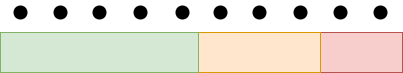
As a simple example, suppose that a group of people are surveyed regarding their favorite flavor of ice cream, as in Figure 1.

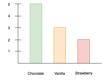
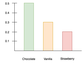
We can then compute a probability distribution (as a "probability mass function") by normalizing the histogram from Figure 1 by dividing each tally by the sum of all people surveyed (10), as in Figure 2.

Suppose that we wish to draw random samples from this distribution. One method of doing so involves computing the inverse of the cumulative distribution. The cumulative distribution is depicted in Figure 3. If we impose an arbitrary total ordering on the flavors (e.g. chocolate is first, vanilla is second, strawberry is third, as depicted from left to right in the figure), then the cumulative distribution tells us the probability that a flavor is less than or equal to the respective flavor.

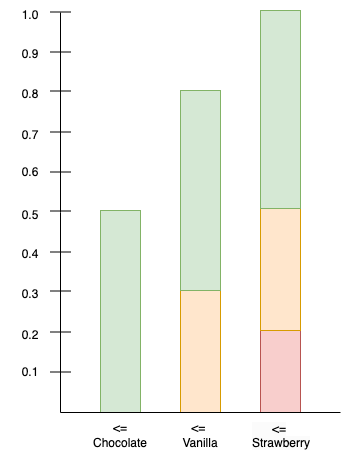
We can then compute the inverse of the cumulative distribution, which accepts a number \(u\) in the range \([0,1]\) and outputs a flavor:

\[F^{-1}(u) = \begin{cases}\text{chocolate} & \text{if}~0 \le u \le 0.5, \\ \text{vanilla} & \text{if}~0.5 \lt u \le 0.8, \\ \text{strawberry} & \text{if}~0.8 \lt u \le 1.0\end{cases}\]

If we generate a random number \(u \in [0, 1]\) (for instance, using a pseudo-random number generator on a computer), then we can sample a flavor using the inverse cumulative distribution function:

\[F^{-1}(u).\]

If the generated random numbers are uniformly distributed, then we will sample flavors proportionally, as is depicted in Figure 4.

There are other methods of sampling distributions, such as rejection sampling. In the case of discrete (finite) random variables, sampling a distribution is relatively straightforward. However, in general, sampling from a distribution is a difficult problem.

The Metropolis-Hastings algorithm is an ingenious technique for sampling a wide class of distributions: it constructs a Markov chain one step at a time, such that the stationary distribution of the chain is equal to the target distribution, and can do so only by evaluating a function which is proportional to the target distribution. At each step, the algorithm maintains the most recent sample and proposes a candidate sample and determines whether to accept or reject the given proposal based on a simple criterion.

However, as the term chain implies, the original algorithm can only generate samples sequentially, which is a serious problem when implementing the algorithm in a parallel manner, for instance on a GPU. The typical solution is to use multiple chains; however, this means that the chains are independent and "shorter" (consist of fewer steps, affording less opportunity to converge to the stationary distribution), and there is overhead, such as storage, associated with each chain, so using multiple chains can result in serious drawbacks.

However, there are generalizations of the Metropolis-Hastings algorithm which are amenable to parallelization and do not suffer any drawbacks. This post will discuss one particular such generalization which generates multiple independent proposals at each step (hence permitting the proposals to be generated in parallel), and then utilizes all proposals (not just the single accepted proposal, if any) by weighting them in an appropriate manner which preserves the stationary distribution and even reduces variance.

Papers

The algorithm which will be discussed in this post is described in the paper "Rao-Blackwellised parallel MCMC" [1] by authors Tobias Schwedes and Ben Calderhead (referred to as "RB-MP-MCMC" there). The earlier paper "A general construction for parallelizing Metropolis−Hastings algorithms" [2] by author Ben Calderhead also describes aspects of this algorithm. The algorithm is based on earlier work described in the paper "Using All Metropolis-Hastings Proposals to Estimate Mean Values" [3] by author Håkon Tjelmeland.

The original algorithm is described in the paper "Equation of State Calculations by Fast Computing Machines" [4] by Nicholas Metropolis which was extended in the paper "Monte Carlo Sampling Methods Using Markov Chains and Their Applications" [5] by W.K. Hastings (hence the name "Metropolis-Hastings").

See the references at the end of the post.

Before proceeding, a brief overview of probability theory is needed in order to establish the basic terminology and concepts.

Measures

Our goal is to assign a probability to certain sets (where we think of the sets as particular events). In order to do so, we must establish which sorts of sets are measurable.

A collection \(\Sigma\) of subsets of a set \(X\) is called a \(\mathbf{\sigma}\)-algebra if it contains \(X\) and is closed under complements and countable unions, i.e.:

• \(X \in \Sigma\),
• \(X \setminus A \in \Sigma\) for all \(A \in \Sigma\),
• \(\cup \mathcal{F} \in \Sigma\) for any countable family of sets \(\mathcal{F} \subseteq \Sigma\).

The elements \(A \in \Sigma\) are called measurable sets and the pair \((X, \Sigma)\) is called a measurable space.

Given two measurable spaces \((X, \Sigma)\) and \((Y, T)\), a function \(f : X \rightarrow Y\) is called a measurable function if \(f^{-1}(E) \in \Sigma\) for every \(E \in T\).

Given a measurable space \((X, \Sigma)\), a measure is a map \(\mu : X \rightarrow [0, \infty]\) (i.e. to the non-negative portion of the extended real line) such that the following properties are satisfied:

• \(\mu(\emptyset) = 0\),
• countable additivity: \(\mu(\cup\mathcal{F}) = \sum_{A \in \mathcal{F}}\mu(A)\) for any countable family of sets \(\mathcal{F} \subseteq \Sigma\).

The triple \((X, \Sigma, \mu)\) is called a measure space.

A measure is called \(\mathbf{\sigma}\)-finite if \(\mu(A) < \infty\) for all measurable sets \(A\).

Given any map \(f : X \rightarrow Y\) between two measurable spaces \((X, \Sigma)\) and \((Y, T)\), for any measure \(\mu : \Sigma \rightarrow [0,\infty]\), the pushforward measure \(f_*(\mu)\) is the measure defined for all \(B \in T\) such that

\[f_*(\mu)(B) = \mu\left(f^{-1}(B)\right).\]

Probability Spaces

If \(\mu(X) = 1\), then the measure space is called a probability space. A probability space is typically denoted \((\Omega, \mathcal{F}, P)\), i.e. it consists of the following data:

• A set \(\Omega\) called the sample space whose elements are called outcomes,
• A \(\sigma\)-algebra \(\mathcal{F}\) consisting of subsets of the outcomes called the event space whose elements are called events,
• A probability measure \(P\).

Thus, each event is a measurable set of outcomes, and the measure assigned to it is called its probability.

For instance, the sample space representing the outcome of the roll of a die could be represented by \(\{1,2,3,4,5,6\}\) and the event \(\{2,4,6\}\) could represent a roll landing on an even-numbered face, whose probability is \(P(\{2,4,6\}) = 1/2\).

Events are sets because sets represent arbitrary predicates (they are the extension of the predicate, i.e. \(\{\omega \in \Omega \mid \phi(\omega)\}\)). Thus, events can encode arbitrary predicates such as "the roll of two even number dies and one odd-numbered dice", etc.

The conditional probability \(P(A \mid B)\), which represents the probability of an event \(A\) occurring given that an event \(B\) has occurred, is defined as

\[P(A \mid B) = \frac{P(A \cap B)}{P(B)}.\]

Random Variables

Given a probability space \((\Omega, \mathcal{F}, P)\) and a measurable space \((E, \Sigma)\), a random variable is a measurable function \(X : \Omega \rightarrow E\).

Random variables are functions, but they are often written in abbreviated notation. For instance, the probability that a random variable occupies a value in a measurable set \(A \subseteq E\) is often written as follows:

\[P(X \in A) = P(\{\omega \in \Omega \mid X(\omega) \in A\}).\]

As another example, the probability that a random variable occupies a distinct value is often written as follows:

\[P(X = a) = P(\{\omega \in \Omega \mid X(\omega) = a\}).\]

As another example, if the set \(E\) is an ordered set with relation \(\le\), then the following notation is often used:

\[P(X \le a) = P(\{\omega \in \Omega \mid X(\omega) \leq a\}).\]

In general, for any appropriate predicate \(\phi\), the following notation is used:

\[P(\phi(X)) = P(\{\omega \in \Omega \mid \phi\left(X(\omega)\right)).\]

The distribution (or probability distribution) of a random variable \(X\) is the pushforward measure with respect to \(X\), and is thus defined, for all \(A \in \Sigma\) as

\[X_*(P)(A) = P(X^{-1}(A)) = P(\{\omega \in \Omega \mid X(\omega) \in A\}) = P(X \in A).\]

A real-valued random variable is a random variable whose codomain is \(\mathbb{R}\), i.e. a map \(X : \Omega \rightarrow \mathbb{R}\) (typically, the Borel \(\sigma\)-algebra \(\mathcal{B}(\mathbb{R})\) is implied, which is the smallest \(\sigma\)-algebra containing all the open intervals in \(\mathbb{R}\)).

The cumulative distribution function (CDF) of a real-valued random variable \(X\) is the function \(F_X\) defined by

\[F_X(x) = P(X \le x) = P(\{\omega \in \Omega \mid X(\omega) \le x\}).\]

The CDF completely characterizes the distribution of a real-valued random variable (i.e. each distribution has a unique CDF and conversely, each CDF corresponds to a unique distribution).

For random variables on discrete (finite or countable) measurable spaces, the probability mass function (PMF) \(p_X\) is defined so that

\[p_X(x) = P(X = x).\]

Each real-valued random variable generates a \(\sigma\)-algebra. The \(\mathbf{\sigma}\)-algebra generated by a random variable \(X\) with values in a measurable space \((E, \Sigma)\) is denoted \(\sigma(X)\) and is defined as follows:

\[\sigma(X) = \{X^{-1}(A) \mid A \in \Sigma\}.\]

Although probability spaces and random variables are important for theoretical purposes, the distribution of random variables is typically what matters, and so the probability space and random variables are suppressed (they are not defined explicitly). There might be many random variables defined on various probability spaces which exhibit the same distribution; it is the distribution itself that is important. There are theoretical results guaranteeing the existence of suitable probability spaces and random variables for a given distribution. Thus, generally, the distribution is used, typically via a CDF or PDF (see below).

Integrals

Given a real-valued measurable function \(f : X \rightarrow Y\) on measurable spaces \((X, \Sigma)\) and \((Y, T)\), it is possible to define the (Lebesgue) integral of \(f\) over a measurable set \(E \in \Sigma\) with respect to a measure \(\mu\) on \(\Sigma\), denoted

\[\int_E f~d\mu.\]

The same integral is sometimes denoted

\[\int_E f(x)~d\mu(x)\]

or as

\[\int_E f(x)~\mu(dx).\]

Consider Figure 5.

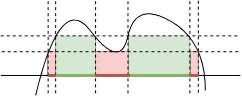
An indicator function \(1_S : X \rightarrow \{0, 1\}\) (also written \(\mathbb{1}_S\)) of a measurable set \(S\) is defined such that

\[1_S(x) = \begin{cases}1 & \text{if } x \in A,\\ 0 & \text{otherwise}.\end{cases}\]

The integral of an indicator function is defined as follows:

\[\int 1_S ~d\mu = \mu(S).\]

A finite linear combination \(s\) of indicator functions is called a simple function:

\[s = \sum_k a_k 1_{S_k},\]

where \(a_k \in \mathbb{R}\) the \(S_k\) are disjoint measurable sets. When each of the coefficients \(a_k\) are positive, the integral of a simple function is defined as

\[\int\left( \sum_k a_k1_{S_k}\right)~d\mu = \sum_k a_k ~\int 1_{S_k}~d\mu = \sum_k a_k \mu(S_k).\]

If \(E\) is a measurable subset of \(X\), then the integral over this domain is defined as

\[\int_E s~d\mu = \int 1_E \cdot s~d\mu = \sum_k a_k ~\mu(S_k \cap E).\]

Then, the integral of a non-negative measurable function \(f : X \rightarrow \mathbb{R}\) is defined as the supremum of the integrals of all non-negative simple functions bounded by \(f\):

\[\int_E f~d\mu = \sup\left\{ \int_E s~d\mu \mid 0 \le s \le f, s ~\text{simple} \right\}.\]

We can then define non-negative measurable functions as follows:

\[f^+(x) = \begin{cases}f(x) & \text{if } f(x) \gt 0,\\ 0 & \text{otherwise}\end{cases},\]

and

\[f^-(x) = \begin{cases}-f(x) & \text{if } f(x) \lt 0,\\ 0 & \text{otherwise}\end{cases}.\]

Then \(|f| = f^+ - f^-\). If at least one of \(\int f^+~d\mu\) or \(\int f^-~d\mu\) is finite, then the integral is said to exist, and is then defined as

\[\int f~d\mu = \int f^+~d\mu - \int f^-~d\mu,\]

and if

\[\int |f|~d\mu < \infty,\]

the function is said to be integrable.

Some details (such as assumptions regarding \(\infty\)) have been ignored, but this gives the general idea of the integral.

Densities

The Radon-Nikodym Theorem is an important result in measure theory which states that, for any measurable space \((X, \Sigma)\) on which two measures \(\mu\) and \(\nu\) are defined (subject to certain conditions, namely, that both measures are \(\sigma\)-finite and \(\nu \ll \mu\), that is, \(\nu\) is absolutely continuous with respect to \(\mu\)), there exists a \(\Sigma\)-measurable function \(f : X \rightarrow [0,\infty)\), such that for any measurable set \(A \in \Sigma\),

\[\nu(A) = \int_A f~d\mu.\]

The function \(f\) thus represents a density of one measure with respect to another. Because of the formal analogy to the fundamental theorem of calculus, such a density is often called a "derivative" (although it is not related to the usual concept of a derivative, namely, the best linear approximation of a continuous function), and is denoted

\[\frac{d \nu}{d \mu},\]

so that

\[\nu(A) = \int_A \frac{d \nu}{d \mu}~d\mu.\]

A probability density function (PDF) of a random variable \(X\) with values in a measurable set \((E, \Sigma)\) is any density \(f\) of the corresponding distribution with respect to a reference measure \(\mu\), i.e.

\[f = \frac{dX_*P}{d\mu},\]

and hence, for any measurable set \(A \in \Sigma\),

\[P(X \in A) = \int_{X^{-1}(A)}dP = \int_A f~d\mu.\]

The distribution of a real-valued random variable admits a density function if and only if its CDF is absolutely continuous; in this case, the derivative of the CDF is a PDF:

\[\frac{d}{dx}F_X(x) = f(x).\]

Stochastic Processes

Given a probability space \((\Omega, \mathcal{F}, P)\) and a measurable space \((\mathcal{S}, \Sigma)\), a stochastic process is a collection of \(\mathcal{S}\)-valued random variables indexed by some set \(T\) (typically, \(T = \mathbb{N}\), resulting in a sequence of random variables):

\[\{X_t : t \in T\}.\]

The set \(T\) is called the index set and the set \(\mathcal{S}\) is called the state space. The indices \(t \in T\) are often referred to as times.

A stochastic process is stationary if each of its random variables have the same distribution.

Filtrations

Given a \(\sigma\)-algebra \(\mathcal{F}\) and a totally-ordered index set \(I\) (e.g. \(\mathbb{N}\)), a sequence of \(\sigma\)-algebras

\[\left(\mathcal{F}_i\right)_{i \in I}\]

such that \(\mathcal{F}_i \subseteq \mathcal{F}\) (i.e. each is a sub-algebra) is called a filtration if \(\mathcal{F}_i \subseteq \mathcal{F}_j\) whenever \(i \leq j\).

A stochastic process \((X_i)_{i \in I}\) defined for a probability space \((\Omega, \mathcal{F}, P)\) with values in a measurable space \((S, \Sigma)\) is adapted to the filtration if each random variable \(X_i : \Omega \rightarrow S\) is a measurable function with respect to the measurable space \((\Omega, \mathcal{F}_i)\).

Intuitively, a filtration models the information gathered from a stochastic process up to a particular point in the process.

Expectations

If \(X\) is an integrable real-valued random variable on a probability space with probability measure \(P\), then the expectation (or mean) of \(X\) is denoted \(E(X)\) and is defined as follows:

\[E(X) = \int X ~dP.\]

For each event \(A\), the mapping \(P(- \mid A)\) is also a probability measure. The conditional expectation of a real-valued random variable \(X\) with respect to an event \(A\) is defined as

\[E(X \mid A) = \int X(\omega) P(d\omega \mid A).\]

The conditional expectation of a real-valued random variable \(X\) with respect to a \(\sigma\)-algebra \(\mathcal{F}\) is a random variable denoted \(E(X \mid \mathcal{F})\) which satisfies the following properties:

• \(E(X \mid \mathcal{F})\) is \(\mathcal{F}\)-measurable
• For each \(A \in \mathcal{F}\), \(E(1_AX) = E(1_AE(X \mid \mathcal{F}))\).

The conditional probability of an event \(A\) given a \(\sigma\)-algebra \(\mathcal{F}\) is defined as follows:

\[P(A \mid \mathcal{F}) = E(1_B \mid \mathcal{F}).\]

Likewise, the conditional expectation of a real-valued random variable \(X\) with respect to another real-valued random variable \(Y\) is defined as

\[E(X \mid Y) = E(X \mid \sigma(Y)).\]

Markov Processes

A stochastic process \((X_t)_{t \in T}\) indexed on a set \(T\) on a probability space \((\Omega, \mathcal{F}, P)\) with values in a measurable space \((S, \Sigma)\) which is adapted to a filtration \((\mathcal{F}_t)_{t \in T}\) is a Markov process if, for all \(A \in \Sigma\) and each \(s,t \in T\) with \(s \lt t\),

\[P(X_t \in A \mid \mathcal{F}_s) = P(X_t \in A \mid X_s).\]

This property is called the Markov property.

Intuitively, the Markov property indicates that a Markov process only depends on the most recent state, not on the entire history of prior states.

A Markov process is time-homogeneous if, for all \(s,t \in T\), \(x \in A\), and \(A \in \Sigma\),

\[P(X_{s+t} \in A \mid X_t = x) = P(X_t \in A \mid X_0 = x).\]

This property indicates that the transition probability is independent of time (i.e. is the same for all times).

A Markov process is called a discrete-time process if \(T = \mathbb{N}\).

Given measurable spaces \((\Omega_1, \mathcal{A}_1)\) and \((\Omega_2, \mathcal{A}_2)\), a transition kernel is a map \(\kappa : \Omega_1 \times \mathcal{A}_2 \rightarrow [0, \infty]\) such that that following properties hold:

• \(\kappa(-, A_2)\) is a measurable map with respect to \(\mathcal{A}_1\) for every \(A_2 \in \mathcal{A}_2\),
• \(\kappa(\omega_1, -)\) is a \(\sigma\)-finite measure on \((\Omega_2, \mathcal{A}_2)\) for every \(\omega_1 \in \Omega_1\).

If a stochastic kernel is a probability measure for all \(\omega_1 \in \Omega_1\), the \(\kappa\) is called a stochastic kernel or Markov kernel.

Markov Chains on Arbitrary State Spaces

A discrete-time, time-homogeneous Markov process consisting of real-valued (or real-vector-valued) random variables, for our purposes, will be called a Markov chain (although other types of Markov processes are also called Markov chains).

The initial distribution \(\pi_0\) of a Markov chain is the distribution of the first random variable \(X_0\), i.e., for all \(A \subseteq \mathcal{S}\),

\[\pi_o(A) = X_*(P)(A) = P(X \in A).\]

We can then define a stochastic kernel \(p\) as follows:

\[p(x, A) = P(X_{s+t} \in A \mid X_t = x) = P(X_t \in A \mid X_0 = x).\]

Since a Markov chain is time-homogeneous, this is well-defined.

The distribution \(\pi_1\) of \(X_1\) can then be expressed in terms of the distribution \(\pi_0\) as follows:

\[\pi_1(A) = P(X_1 \in A) = \int_{x \in \mathcal{S}}p(x,A)~d\pi_0(x).\]

Likewise, the distribution \(\pi_t\) at each time \(t\) can be defined recursively as follows:

\[\pi_t(A) = P(X_t \in A) = \int_{x \in \mathcal{S}}p(x,A)~d\pi_{t-1}(x).\]

If the random variables admit densities, then \(X_1\) has probability density \(f_1\) such that

\[\pi_1(A) = \int_{x \in A}f_1(x)~dx.\]

Likewise, the transition kernel can be expressed in terms of a conditional density \(f(x_t \mid x_{t-1})\) as follows:

\[p(x_{t}, A) = \int_{x_n \in A}f(x_t \mid x_{t-1})~dx_t.\]

Then, each of the densities can be expressed as follows:

\[\pi_t(A) = \int_{x_{t-1}}f(x_t \mid x_{t-1})f(x_{t-1})~dx_{t-1}.\]

If the Markov process has a stationary distribution, that is, if each of the random variables has the same distribution \(\pi\) (and hence the same as the initial distribution \(\pi_0 = \pi\)), then the distribution at any time \(t\) may be expressed as

\[\pi(A) = \int_{x \in \mathcal{S}}p(x,A)~d\pi(x).\]

This equation is called the balance equation.

In terms of PDFs, the balance equation is expressed as

\[f(y) = \int_{x \in \mathcal{S}}f(y \mid x)f(x)~dx.\]

A Markov chain satisfies detailed balance if there exists a probability measure \(\pi\) with density \(f\) such that for all \(x,y \in \mathcal{S}\),

\[f(y \mid x) f(x) = f(x \mid y) f(y).\]

Then, integrating both sides, we obtain

\[\int_{y \in \mathcal{S}}f(y \mid x) f(x) ~dy = \int_{y \in \mathcal{S}} f(x \mid y) f(y) ~dy.\]

Thus,

\[f(x) \int_{y \in \mathcal{S}}f(y \mid x) ~dy = \int_{y \in \mathcal{S}} f(x \mid y) f(y) ~dy,\]

and, since

\[ \int_{y \in \mathcal{S}}f(y \mid x)~dy = 1,\]

it follows that

\[f(x) = \int_{y \in \mathcal{S}} f(x \mid y) f(y) ~dy.\]

This is (with an appropriate change of variables) exactly the balance equation. Thus, detailed balance implies balance, i.e. it implies that \(\pi\) is a stationary distribution.

Example Markov Chain on a Finite State Space

It is instructive to consider an example of a Markov chain on a finite state space. We will work with the distributions, via the probability mass function (PMF) and cumulative distribution function (CDF).

Consider the following Markov chain:

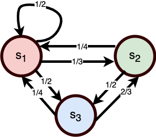
• The state space \(\mathcal{S}\) consists of three states \(\mathcal{S} = \{s_1, s_2, s_3\}\),
• The initial distribution \(\pi_0\) defined such that \(\pi_0(s_1) = 1/2\), \(\pi_0(s_2) = 1/4\), and \(\pi_0(s_3) = 1/4\)
• The transition function \(P\) is defined so that \(P(s_j \mid s_i)\) is given by the labels on the arrows from state \(s_i\) to state \(s_j\) in Figure 6.

A Markov chain on a finite state space can be conceived as a state machine with probabilistic transitions, as in Figure 6.

Next, define the inverse CDF \(F^{-1}_0\) corresponding to \(\pi_0\):

\[F^{-1}_0(u) = \begin{cases}s_1 & \text{if}~ 0 \le u \le \frac{1}{2} \\ s_2 & \text{if}~ \frac{1}{2} \lt u \le \frac{3}{4} \\ s_3 & \text{if}~ \frac{3}{4} \lt u \le 1.\end{cases}\]

We can then sample a state by generating a uniformly distributed random number \(u_0 \in [0,1]\). Suppose that \(u_0 = 0.84\). Then \(F^{-1}_0(u_0) = s_3\), and so the initial state is \(s_3\).

Then, we can define the next distribution \(\pi_1\) as follows:

\[\pi_1(s) = \sum_{i=1}^3 \pi_0(s_i)P(s \mid s_i).\]

This uses the Law of Total Probability, i.e. the probability of occupying a given state \(s\) at time \(t=1\) is the probability of occupying some state \(s_i\) at time \(t = 0\) and then transitioning to state \(s\). Thus, we compute \(\pi_1(s_1) = 11/24\), \(\pi_1(s_2) = 1/4\), \(\pi_1(s_3) = 7/24\).

We can then define the next inverse CDF \(F^{-1}_1\) corresponding to \(\pi_1\) as follows:

\[F^{-1}_1(u) = \begin{cases}s_1 & \text{if}~ 0 \le u \le \frac{11}{24} \\ s_2 & \text{if}~ \frac{11}{24} \lt u \le \frac{17}{24} \\ s_3 & \text{if}~ \frac{17}{24} \lt u \le 1.\end{cases}\]

We can then sample the next state by generating a uniformly distributed random number \(u_1 \in [0,1]\). Suppose that \(u_1 = 0.08\). Then, \(F^{-1}_1(u_1) = s_1\), and so the next state is \(s_1\).

This process can continue indefinitely. We can define the distribution \(\pi_t\) at time \(t+1\) recursively as follows:

\[\pi_{t+1}(s) = \sum_{i=1}^3 \pi_t(s_i)P(s \mid s_i).\]

If the Markov chain possesses a stationary distribution, then it will be the limit as \(t \to \infty\). The stationary distribution will satisfy

\[\pi(s) = \sum_{i=1}^3 \pi(s_i)P(s \mid s_i).\]

Each distribution \(\pi_t\) can be represented as a row vector. For instance,

\[\pi_0 = \begin{bmatrix}\frac{1}{2} & \frac{1}{4} & \frac{1}{4}\end{bmatrix}.\]

Likewise, the transition function can be represented as a matrix \(P_{ij} = P(s_j \mid s_i)\) as follows:

\[P_{ij} = \begin{bmatrix}\frac{1}{2} & \frac{1}{3} & \frac{1}{2} \\ \frac{1}{4} & 0 & \frac{1}{2} \\ \frac{1}{4} & \frac{2}{3} & 0\end{bmatrix}.\]

Then, each distribution \(\pi_{t+1}\) can be computed via the recursive equation

\[\pi_{t+1} = \pi_tP.\]

Expanding this recursive equation yields an iterative equation:

\begin{align}\pi_{t+1} &= \pi_tP \\&= (\pi_{t-1}P)P \\&= \dots \\&= \pi_0P^t.\end{align}

If the Markov chain possesses a stationary distribution \(\pi\), then it will satisfy

\[\pi = \pi P.\]

If we write

\[\pi =\begin{bmatrix}x & y & z\end{bmatrix},\]

then this yields the equation

\[\begin{bmatrix}x & y & z\end{bmatrix} =\begin{bmatrix}x & y & z\end{bmatrix}\begin{bmatrix}\frac{1}{2} & \frac{1}{4} & \frac{1}{4} \\ \frac{1}{3} & 0 & \frac{2}{3} \\ \frac{1}{2} & \frac{1}{2} & 0\end{bmatrix}.\]

We must additionally impose the constraint that \(x +y + z = 1\) since these represent probabilities. This then corresponds to the augmented system of equations

\begin{align}\frac{1}{2}x &+ \frac{1}{4}y & + \frac{1}{4}z &= x \\ \frac{1}{3}x & & + \frac{2}{3}z &= y \\ \frac{1}{2}x & + \frac{1}{2}y & &= z \\ x & + y & + z & = 1.\end{align}

Solving this yields \(x = 1/3\), \(y = 1/3\), \(z = 1/3\). So, the stationary distribution is a uniform distribution.

The Rao-Blackwell Theorem

The term parameter refers to a quantity that summarizes some detail of a statistical population, such as the mean, or standard deviation of the population, and is often denoted \(\theta\). A statistic is a random variable \(X\) which represents some observable quantity. An estimator for a parameter is an observable random variable \(\hat{\theta}(X)\) used to estimate \(\theta\). A sufficient statistic is a statistic \(T(X)\) such that the conditional probability of \(X\) given \(T(X)\) does not depend on \(\theta\).

The mean-squared error (MSE) of an estimator \(\hat{\theta}\) for a parameter \(\theta\) is defined as

\[\mathbb{E}((\hat{\theta} - \theta)^2).\]

The Rao-Blackwell estimator \(\tilde{\theta}\) is the conditional expected value of an estimator for a parameter \(\theta\) given a sufficient statistic \(T(X)\), namely

\[\tilde{\theta} = \mathbb{E}(\hat{\theta}(X) \mid T(X)).\]

One version of the Rao-Blackwell theorem states that the mean-squared error of the Rao-Blackwell estimator does not exceed that of the original estimator, namely

\[\mathbb{E}((\tilde{\theta} - \theta)^2) \le \mathbb{E}((\hat{\theta} - \theta)^2).\]

Another version states that the variance of the Rao-Blackwell estimator is less than or equal to the variance of the original estimator.

The Rao-Blackwell theorem can be applied to produce improved estimators. In particular, it will provide a means of using the rejected samples produced by the Metropolis-Hastings algorithm.

The Metropolis-Hastings Algorithm

The Metropolis-Hastings algorithm, like all MCMC techniques, designs a Markov chain such that the stationary distribution \(\pi\) of the chain is some desired distribution, called the target distribution. The distribution of the chain asymptotically approaches the stationary distribution, and the sequence of states generated by the chain can be used as samples from the target distribution. Here, we represent distributions via PDFs.

A Markov chain is characterized by its transition probability \(P(x_i \mid x_j)\). The algorithm proceeds by designing \(P(x_i \mid x_j)\) such that the stationary distribution is \(\pi\).

First, the condition of detailed balance is imposed, namely.

\[P(x_i \mid x_j)\pi(x_j) = P(x_j \mid x_i)\pi(x_i),\]

which guarantees the balance condition

\[\pi(x_i) = \int P(x_i \mid x_j)\pi(x_j)~dx_j.\]

Then, the transition distribution \(P\) is decomposed into two distributions, the acceptance distribution \(A(x_i \mid x_j) \in [0, 1]\) which represents the probability of accepting state \(x_i\) given state \(x_j\), and the proposal distribution \(K(x_i \mid x_j)\) which represents the probability of proposing a transition from \(x_i\) to \(x_j\). The transition distribution is then defined as the product of these distributions:

\[P(x_i \mid x_j) = K(x_i \mid x_j)A(x_i \mid x_j).\]

The detailed balance condition then implies that

\[\pi(x_j)K(x_i \mid x_j)A(x_i \mid x_j) = \pi(x_i)K(x_j \mid x_i)A(x_j \mid x_i),\]

which further implies that

\[\frac{A(x_j \mid x_i)}{A(x_i \mid x_j)} = \frac{\pi(x_j)K(x_i \mid x_j)}{\pi(x_i)K(x_j \mid x_i)}.\]

Often, the proposal distribution is designed to be symmetric, meaning that

\[K(x_i \mid x_j) = K(x_j \mid x_i),\]

and so this simplifies to

\[\frac{A(x_j \mid x_i)}{A(x_i \mid x_j)} = \frac{\pi(x_j)}{\pi(x_i)}.\]

The typical choice for the acceptance distribution is

\[A(x_i \mid x_j) = \mathrm{min}\left(1, \frac{\pi(x_j)K(x_i \mid x_j)}{\pi(x_i)K(x_j \mid x_i)}\right).\]

Then, either \(A(x_i \mid x_j) = 1\) or \(A(x_j \mid x_i) = 1\) and the detailed balance equation will be satisfied.

Thus, the balance equation is also satisfied, and the stationary distribution of the chain will be the target distribution \(\pi\).

Note that since the probability of acceptance is \(A(x_i \mid x_j)\), the probability of rejection is therefore \(1 - A(x_i \mid x_j)\).

Detailed balance guarantees the existence of a stationary distribution; the uniqueness of the stationary distribution is guaranteed under certain conditions (the ergodicity of the chain).

This yields a concrete algorithm:

1. Choose an initial state \(x_0\). Set time \(t = 0\). Set \(x_t = x_0\).
2. Iterate:
   1. Generate a random proposal state \(x'\) by sampling from the distribution \(K(x' \mid x_t)\).
   2. Either accept the proposal or reject the proposal.
      1. Generate a uniformly distributed random number \(u\) in the range \([0,1]\).
      2. If \(u \le A(x' \mid x_j)\), then accept the proposal state: set \(x_{t+1} = x'\).
      3. If \(u > A(x' \mid x_j\), then reject the proposal state: set \(x_{t+1} = x_t\) (i.e. accept the current state).
   3. Continue at time \(t+1\).

This algorithm will yield a sequence of states which represent samples from the target distribution.

Note that the proposal state is not used when it is rejected; it is possible to use it, however. We will return to this issue in the discussion of the Rao-Blackwell theorem.

A New Perspective on Metropolis-Hastings

A change in the perspective of the Metropolis-Hastings algorithm will indicate its potential generalization. The algorithm can be conceived in terms of an auxiliary Markov chain. The proposal state and the current state comprise the states of a two-state auxiliary Markov chain whose transition probabilities are given by the acceptance probabilities \(A(x_i \mid x_j)\) as in Figure 7.

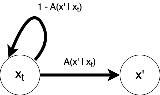
A new auxiliary chain is constructed during each iteration of the algorithm. The chain begins in state \(x_t\). Acceptance of the proposal state \(x'\) corresponds to a transition \(x_t \rightarrow x'\) which has probability \(A(x' \mid x_t)\) and rejection of the proposal state (or acceptance of the current state) corresponds to a transition \(x_t \rightarrow x'\), which implicitly has probability \(1 - A(x' \mid x_t\). The acceptance probability \(A\) thus implicitly represents the transition probability of this auxiliary Markov chain. Thus, simulating this auxiliary Markov chain for a single step represents accepting or rejecting the proposal state.

We refer to the original Markov chain described explicitly in the Metropolis-Hastings algorithm as the primary chain to distinguish it from this implicit auxiliary chain.

This shift in perspective indicates several avenues toward generalization:

1. A different auxiliary Markov chain can be constructed, in particular, one with multiple proposal states.
2. The auxiliary Markov chain can be simulated for more than one step.

However, it is essential to ensure that the stationary distribution of the Markov chain is preserved.

In this post, we will not consider simulating the auxiliary chain for more than one step (but see references [1] and [2] for more information on this approach). This is less amenable to parallelization since it incurs significant coordination overhead. Instead, we will consider an auxiliary Markov chain with multiple proposal states which is simulated only once, yet each of the proposals is utilized via a Rao-Blackwell estimator. This approach allows the proposals to be computed in parallel, and minimizes the coordination needed.

Multiple Proposal Metropolis-Hastings

As in the single proposal case, we have a target distribution which is continuous on \(\mathbb{R}^n\) with density \(\pi\).

Logically, we think of the process as follows: at each iteration of the Metropolis-Hastings algorithm, we produce an auxiliary Markov chain consisting of multiple proposal states, then we simulate the auxiliary chain for a single step to select the next state.

Just as in the single-proposal algorithm, we will maintain a single current state at each step of the process. However, we will propose an entire vector of proposals at each step.

We thus need to define the proposal density of a proposal vector given the current state.

First, denote the number of proposals as \(N\), where \(N \ge 1\). Then, let there be a sequence of \(N+1\) states, which include the proposals and current state:

\[y_1, y_2,\dots,y_{N+1}.\]

We then use the notation

\[\mathbf{y} = (y_1,y_2,\dots,y_{N+1}).\]

The notation

\[\mathbf{y}_{\backslash i} = (y_1,\dots,y_{i-1},y_{i+1},\dots,y_m)\]

indicates the projection of \(\mathbf{y}\) which deletes the \(i\)-th component.

We can define a transition kernel \(\tilde{\kappa}\) in terms of the the underlying proposal kernel \(\kappa\) of the Markov chain as

\[\tilde{\kappa}(y_i, \mathbf{y}_{\backslash i}) = \prod_{j \ne i}\kappa(y_i, y_j).\]

We can then define a multiple proposal density \(p_i\) for each \(1 \le i \le N+1\) in terms of the target distribution \(\pi\) as

\[p_i(\mathbf{y}) = \pi(y_i)\tilde{k}(y_i,\mathbf{y}_{\backslash i}).\]

Next, define a uniformly-distributed auxiliary random variable \(I\) with values in the set \(\{1, \dots, N+1\}\). This random variable indicates which of the proposal densities to use (which index to use). Since it is uniformly distributed, each index has probability \(1/(N+1)\).

Next, define a joint distribution as follows

\[p(\mathbf{y}, i) = \frac{1}{N + 1}p_i(\mathbf{y}).\]

Finally, denote the transition matrix of the auxiliary chain as

\[A(i, j) = [A_{ij}].\]

There will be a different transition matrix for each auxiliary chain, and each auxiliary chain corresponds to a different proposal vector.

We can now formulate the analog of the balance condition for the auxiliary chain:

\[p_i(\mathbf{y}) = \sum_{j=1}^{N+1} p_j(\mathbf{y})A(j, i).\]

Likewise, there is an analog of the detailed balance condition for the auxiliary chain:

\[p_i(\mathbf{y})A(i, j) = p_j(\mathbf{y})A(j, i).\]

In analogy to the single-proposal algorithm, the following transition matrix is used (which represents the acceptance distribution):

\[A(i,j) = \begin{cases}\frac{1}{N+1}\mathrm{min}\left(1, \frac{p_j(\mathbf{y})}{p_i(\mathbf{y})}\right) & \text{if}~i \neq j \\ 1 - \sum_{k \neq i} A(i,k) & \text{if}~i=j.\end{cases}\]

This transition matrix satisfies the balance equation. To see this, first denote the number of times \(p_i(\mathbf{y})/p_j(\mathbf{y}) \le 1\) as \(k\) and the number of times \(p_i(\mathbf{y})/p_j(\mathbf{y}) \gt 1\) as \(l\). Then

\begin{align}\sum_{j=1}^{N+1} p_j(\mathbf{y})A(j, i) &= \sum_{j \neq i}p_j(\mathbf{y})A(j, i) + p_i(\mathbf{y})A(i,i) \\&= \left(\frac{k}{N+1}p_i(\mathbf{y}) + \frac{l}{N+1}p_j(\mathbf{y})\right) + p_i(\mathbf{y})\left(1 - \sum_{j \neq i}A(i,j)\right) \\&= \left(\frac{k}{N+1}p_i(\mathbf{y}) + \frac{l}{N+1}p_j(\mathbf{y})\right) + p_i(\mathbf{y}) - \left(\frac{k}{N+1}p_i(\mathbf{y}) + \frac{l}{N+1}p_j(\mathbf{y})\right) \\&= p_i(\mathbf{y}). \end{align}

Preservation of Stationary Distribution

Now that we have defined the setting for multiple-proposal Markov chains, we need to establish several essential properties. First, the stationary distribution of the modified Markov process must be preserved, i.e. must still be equal to the target distribution \(\pi\).

The following proof is adapted from appendix A of reference [1].

The notation

\[d\mathbf{y} = dy_1\dots dy_{N+1}\]

and

\[d\mathbf{y}_{\backslash i} = dy_1\dots dy_{i-1}dy_{i+1}\dots dy_{N+1}\]

is used.

First, define a stochastic kernel as follows:

\[P(y_i, B) = \int_{\mathbb{R}^{Nd}}\tilde{k}(y_i, \mathbf{y}_{\backslash i})\sum_{j=1}^{N+1} A(i,j) \mathbb{1}_B(y_j)d\mathbf{y}_{\backslash i}.\]

This kernel indicates the probability that the accepted sample \(y_j\) belongs to a measurable set \(B \in \mathcal{B}(\mathbb{R}^d)\). It can be interpreted as the probability of proposing the proposal vector \(\mathbf{y}_{\backslash i}\) from current state \(y_i\) and then accepting some proposal state \(y_j \in B\).

All transitions from the current state to the next have this form. Thus, we compute, for an arbitrary state \(x = y_i\),

\begin{align}\int_{\mathbb{R}^d}P(x, B)\pi(x)~dx &= \int_{\mathbb{R}^d}\left(\int_{\mathbb{R}^{Nd}}\tilde{k}(y_i, \mathbf{y}_{\backslash i})\sum_{j=1}^{N+1} A(i,j) \mathbb{1}_B(y_j)d\mathbf{y}_{\backslash i}\right)\pi(y_i)~dy_i \\&= \int_{\mathbb{R}^{(N+1)d}}\tilde{k}(y_i, \mathbf{y}_{\backslash i})\sum_{j=1}^{N+1} A(i,j) \mathbb{1}_B(y_j)\pi(y_i)~d\mathbf{y} .\end{align}

For any constant term \(c\), \(\frac{1}{N+1}\sum_1^{N+1} c = c\). Furthermore, since the indices of the formal variables in the integrand are arbitrary (i.e. whether we designate \(y_1\) or \(y_2\), etc. as the current state is irrelevant), re-arranging them does not affect the value of the integral. Thus, we may introduce a summation without affecting the integral as follows:

\begin{align}\int_{\mathbb{R}^{(N+1)d}}\tilde{k}(y_i, \mathbf{y}_{\backslash i})\sum_{j=1}^{N+1} A(i,j) \mathbb{1}_B(y_j)\pi(y_i)~d\mathbf{y} &= \int_{\mathbb{R}^{(N+1)d}}\frac{1}{N+1}\sum_{i=1}^{N+1}\tilde{k}(y_i, \mathbf{y}_{\backslash i})\sum_{j=1}^{N+1} A(i,j) \mathbb{1}_B(y_j)\pi(y_i)~d\mathbf{y}\end{align}

We may then re-associate the terms as follows:

\begin{align}\int_{\mathbb{R}^{(N+1)d}}\frac{1}{N+1}\sum_{i=1}^{N+1}\tilde{k}(y_i, \mathbf{y}_{\backslash i})\sum_{j=1}^{N+1} A(i,j) \mathbb{1}_B(y_j)\pi(y_i)~d\mathbf{y} &= \int_{\mathbb{R}^{(N+1)d}}\frac{1}{N+1}\sum_{j=1}^{N+1}\sum_{i=1}^{N+1}\pi(y_i)\tilde{k}(y_i, \mathbf{y}_{\backslash i}) A(i,j) \mathbb{1}_B(y_j)~d\mathbf{y}.\end{align}

Since the balance condition is satisfied, we then substitute as follows:

\begin{align}\int_{\mathbb{R}^{(N+1)d}}\frac{1}{N+1}\sum_{i=1}^{N+1}\sum_{j=1}^{N+1}\pi(y_i)\tilde{k}(y_i, \mathbf{y}_{\backslash i}) A(i,j) \mathbb{1}_B(y_j)~d\mathbf{y} &= \int_{\mathbb{R}^{(N+1)d}}\frac{1}{N+1}\sum_{j=1}^{N+1}\pi(y_j)\tilde{k}(y_j, \mathbf{y}_{\backslash j}) \mathbb{1}_B(y_j)~d\mathbf{y}.\end{align}

Then, just as before, since the sum does not affect the integral, we may eliminate it as follows:

\begin{align}\int_{\mathbb{R}^{(N+1)d}}\frac{1}{N+1}\sum_{j=1}^{N+1}\pi(y_j)\tilde{k}(y_j, \mathbf{y}_{\backslash j}) \mathbb{1}_B(y_j)~d\mathbf{y} &= \int_{\mathbb{R}^{(N+1)d}}\pi(y_j)\tilde{k}(y_j, \mathbf{y}_{\backslash j}) \mathbb{1}_B(y_j)~d\mathbf{y}.\end{align}

Finally, we re-associate the terms and utilize the fact that \(\tilde{k}\) is a kernel, and thus \(\int_{\mathbb{R}^{Nd}}\tilde{k}(y_i,y_{\backslash i})~d\mathbf{y}_{\backslash i} = 1\) as follows:

\begin{align}\int_{\mathbb{R}^{(N+1)d}}\pi(y_j)\tilde{k}(y_j, \mathbf{y}_{\backslash j}) \mathbb{1}_B(y_j)~d\mathbf{y} &= \int_{\mathbb{R}^d}\pi(y_j)\mathbb{1}_B(y_j)\left(\int_{\mathbb{R}^{(N+1)d}}\tilde{k}(y_j, \mathbf{y}_{\backslash j}) ~d\mathbf{y}_{\backslash j}\right)~dy_j \\&= \int_{\mathbb{R}^d}\pi(y_j)\mathbb{1}_B(y_j)~dy_j \\&= \int_B \pi(x)~dx.\end{align}

Thus, the transition kernel does indeed maintain the stationary distribution.

If we denote the distribution corresponding to the density \(\pi\) as \(\tilde{\pi}\), then the stationary distribution on a Markov process was originally defined as

\[\tilde{\pi}(B) = \int_{\mathcal{S}}P(x,B)~d\tilde{\pi}(x).\]

Noting that

\[\pi = \frac{d\tilde{\pi}}{dx},\]

it follows from the Radon-Nikodym theorem that

\[\int_{\mathcal{S}}P(x,B)~d\tilde{\pi}(x) =\int_{\mathcal{S}}P(x,B) \frac{d\tilde{\pi}}{dx}~dx = \int_{\mathcal{S}}P(x,B) \pi(x) ~dx\]

Likewise, by definition,

\[\tilde{\pi}(B) = \int_B \pi(x)~dx.\]

Thus, the balance equation is satisfied.

The Rao-Blackwell Estimator

MCMC techniques such as the Metropolis-Hastings algorithm are very often used to generate samples for use in numerical integration. When applying MCMC toward numerical integration, the sample mean \(\hat{\mu}\) serves as an estimator for the expected value \(\mathbb{E}_{\pi}[f]\):

\[\frac{1}{N}\sum_{i=1}^N f(x_i) \approx \int f(x) \pi(x)~dx.\]

This is an unbiased estimator (that is, \(\mathbb{E}_{\pi}[\hat{\mu}] = \mathbb{E}_{\pi}[f]\)), since

\begin{align}\mathbb{E}_{\pi}\left[\frac{1}{N}\sum_{i=1}^N f(x_i)\right] &= \frac{1}{N}\sum_{i=1}^N\mathbb{E}_{\pi}[ f(x_i)] \\&= \frac{1}{N}\sum_{i=1}^N \int f(x) \pi(x)~dx \\&= \int f(x) \pi(x)~dx \\&= \mathbb{E}_{\pi}[f].\end{align}

This allows the calculation of arbitrary integrals by using \(f / \pi\) in place of \(f\), in which case

\[\frac{1}{N}\sum_{i=1}^N \frac{f(x_i)}{\pi(x_i)} \approx \int\frac{f(x)}{\pi(x)}\pi(x)~dx = \int f(x)~dx.\]

Our goal is to introduce an alternative estimator \(\tilde{\mu}\) which utilizes all proposals and serves as an unbiased estimator for \(\mathbb{E}_{\pi}[f]\).

We will begin with the sample mean estimator

\[\hat{\mu} = \frac{1}{L}\sum_{l=1}^L f(x^{(l)})\]

and enhance it using the Rao-Blackwell estimator

\[\tilde{\mu} = \mathbb{E}[\hat{\mu} \mid \mathbf{y}^{(l)}].\]

We will proceed by using weighted samples weighted according to weights \(w^{(l)}_i\), where \(1 \le l \le L\) and \(L\) denotes the number of iterations of the algorithm and \(1 \le i \le N + 1\) where \(N\) denotes the number of proposals and hence \(N+1\) indicates the total number of samples including the current sample. The weights must sum to \(1\). Denote the samples (consisting of the current and proposed samples) as \(y^{(l)}_i\).

We define the weights using the acceptance distribution as follows (given current index \(i\)):

\[w^{(l)}_j = A(i, j).\]

The authors in [1] employ the following technique to derive the estimator. First, define the prefix sum of weights \(\eta_i^{(l)}\) as

\[\eta_i^{(l)} = \sum_{j=1}^i w_j^{(l)}.\]

This is related to the CDF of \(A(i,j)\) since the CDF of a PMF is a prefix sum. Therefore, employing the same sampling technique from the introduction, we may sample \(A(i,j)\) by evaluating the inverse of the CDF (the quantile function) with a uniformly distributed random number \(u \sim \mathcal{U}(0, 1)\).

Next, consider the following indicator function:

\[\mathbb{1}_{(\eta_{i-1}^{(l)}, \eta_i^{(l)}]}.\]

Note that, for any \(u \in [0,1]\), \(\mathbb{1}_{(\eta_{i-1}^{(l)}, \eta_i^{(l)}]}(u)\) will evaluate to \(1\) for exactly one index \(i\). Thus, if we denote the accepted sample as \(x^{(l)}\), then, motivated by the inverse CDF sampling technique, we can express \(x^{(l)}\) in terms of \(u^{(l)} \sim\mathcal{U}(0, 1)\) as

\[x^{(l)} = \sum_{i=1}^{N+1}\mathbb{1}_{(\eta_{i-1}^{(l)}, \eta_i^{(l)}]}(u^{(l)})y^{(l)}_i.\]

In fact, this is an expression for the quantile (inverse CDF) function. This is why the sampling technique based on inverse CDFs works: it creates a random variable with the same distribution as another, yet with a different domain.

Thus, the expression is now reformulated on a convenient domain \([0, 1]\) with respect to the uniform (constant) PDF \(p(x) = 1\). The expected value is preserved, but is much easier to compute.

Also note that

\[f(x^{(l)}) = \sum_{i=1}^{N+1}\mathbb{1}_{(\eta_{i-1}^{(l)}, \eta_i^{(l)}]}(u^{(l)})f(y^{(l)}_i).\]

Since these uniformly distributed random numbers are independent of the proposed samples, the conditional expected value of the estimator with respect to the proposed samples is just the expected value of the estimator, namely

\[\mathbb{E}[\hat{\mu} \mid \mathbf{y}^{(l)}] = \mathbb{E}[\hat{\mu}].\]

We then compute

\begin{align}\mathbb{E}\left[f(x^{(l)}) \mid \mathbf{y}\right] &= \mathbb{E}\left[f(x^{(l)})\right] \\&= \mathbb{E}\left[\sum_{i=1}^{N+1}\mathbb{1}_{(\eta_{i-1}^{(l)}, \eta_i^{(l)}]}(u^{(l)})f(y^{(l)}_i)\right] \\&= \int_{(0,1)}\sum_{i=1}^{N+1}\mathbb{1}_{(\eta_{i-1}^{(l)}, \eta_i^{(l)}]}(u^{(l)})f(y^{(l)}_i)~du^{(l)} \\&= \sum_{i=1}^{N+1} \int_{(0,1)}\mathbb{1}_{(\eta_{i-1}^{(l)}, \eta_i^{(l)}]}(u^{(l)})f(y^{(l)}_i)~du^{(l)} \\&= \sum_{i=1}^{N+1} \int_{\eta_{i-1}^{(l)}, \eta_i^{(l)}}f(y^{(l)}_i)~du^{(l)} \\&= \sum_{i=1}^{N+1} \left(\int_{\eta_{i-1}^{(l)}, \eta_i^{(l)}}~du^{(l)}\right)f(y^{(l)}_i) \\&= \sum_{i=1}^{N+1} w^{(l)}_i f(y^{(l)}_i).\end{align}

Each iteration therefore produces the weighted estimate (the Rao-Blackwell estimator)

\[\mathbb{E}[f(x^{(l)}) \mid \mathbf{y}^{(l)}] = \sum_{i=1}^{N+1}w^{(l)}_i f(y^{(l)}_i).\]

The estimator for the mean is thus

\begin{align}\mathbb{E}[\hat{\mu} \mid \mathbf{y}^{(l)}] &= \mathbb{E}[\hat{\mu}] \\&= \mathbb{E}\left[\sum_{l=1}^{L}\frac{1}{L}f(x^{(l)})\right] \\&= \sum_{l=1}^{L} \mathbb{E}\left[f(x^{(l)})\right] \\&= \sum_{l=1}^{L} \sum_{i=1}^{N+1}w^{(l)}_i f(y^{(l)}_i).\end{align}

Unbiased Estimator

Next, we need to demonstrate that this new estimator is unbiased. The following proof is adapted from appendix A of reference [1].

We calculate the expected value with respect to the distribution \(\pi(y_1)\tilde{k}(y_1, \mathbf{y}_{\backslash 1})\) (where \(y_1\) denotes the starting point) as follows:

\begin{align}\mathbb{E}\left[\sum_{i= 1}^{N+1}w^{(l)}_i f(y^{(l)}_i)\right] &= \mathbb{E}\left[ \sum_{i= 1}^{N+1}w^{(l)}_i f(y^{(l)}_i)\right] \\&= \int_{\mathbb{R}^{Nd}}\sum_{i= 1}^{N+1}w^{(l)}_i f(y^{(l)}_i) \pi(y_1)\tilde{k}(y_1, \mathbf{y}_{\backslash 1})~d\mathbf{y}.\end{align}

Then, splitting the sum into two terms, we continue to compute as follows:

\begin{align}\int_{\mathbb{R}^{Nd}}\sum_{i= 1}^{N+1}w^{(l)}_i f(y^{(l)}_i) \pi(y_1)\tilde{k}(y_1, \mathbf{y}_{\backslash 1})~d\mathbf{y} &= \int_{\mathbb{R}^{Nd}}\left(\sum_{i \ne 1}w^{(l)}_i f(y^{(l)}_i) + w^{(l)}_1 f(y^{(l)}_1\right) \pi(y_1)\tilde{k}(y_1, \mathbf{y}_{\backslash 1})~d\mathbf{y} \\&= \left(\sum_{i \ne 1}\int_{\mathbb{R}^{Nd}}w^{(l)}_i f(y^{(l)}_i) \pi(y_1)\tilde{k}(y_1, \mathbf{y}_{\backslash 1})~d\mathbf{y}\right) \\&+ \left(\int_{\mathbb{R}^{Nd}}w^{(l)}_1 f(y^{(l)}_1)\pi(y_1)\tilde{k}(y_1, \mathbf{y}_{\backslash 1})~d\mathbf{y}\right)\end{align}

Since the balance equation states that

\[\sum_{j=1}^{N+1}\pi(y_j)\tilde{\kappa}(y_j, \mathbf{y}_{\backslash j})A(j,i) = \pi(y_i)\tilde{\kappa}(y_i, \mathbf{y}_{\backslash i}),\]

and since \(A(\cdot,i) = w_i\), it follows that

\[\frac{\pi(y_i)\tilde{\kappa}(y_i, \mathbf{y}_{\backslash i})}{\sum_{j=1}^{N+1}\pi(y_j)\tilde{\kappa}(y_j, \mathbf{y}_{\backslash j})} = w_i.\]

We may then infer that

\begin{align}\pi(y_1)\tilde{\kappa}(y_1,\mathbf{y}_{\backslash 1})w_i &= \pi(y_1)\tilde{\kappa}(y_1,\mathbf{y}_{\backslash 1})\frac{\pi(y_i)\tilde{\kappa}(y_i, \mathbf{y}_{\backslash i})}{\sum_{j=1}^{N+1}\pi(y_j)\tilde{\kappa}(y_j, \mathbf{y}_{\backslash j})} \\&= \pi(y_i)\tilde{\kappa}(y_i, \mathbf{y}_{\backslash i})\frac{\pi(y_1)\tilde{\kappa}(y_1,\mathbf{y}_{\backslash 1})}{\sum_{j=1}^{N+1}\pi(y_j)\tilde{\kappa}(y_j, \mathbf{y}_{\backslash j})} \\&= \pi(y_i)\tilde{\kappa}(y_i, \mathbf{y}_{\backslash i})w_1.\end{align}

Substituting this into the prior equation, we obtain

\begin{align}\left(\sum_{i \ne 1}\int_{\mathbb{R}^{Nd}}w^{(l)}_i f(y^{(l)}_i) \pi(y_1)\tilde{k}(y_1, \mathbf{y}_{\backslash 1})~d\mathbf{y}\right) &+ \left(\int_{\mathbb{R}^{Nd}}w^{(l)}_1 f(y^{(l)}_1)\pi(y_1)\tilde{k}(y_1, \mathbf{y}_{\backslash 1})~d\mathbf{y}\right) \\&= \left(\sum_{i \ne 1}\int_{\mathbb{R}^{Nd}}w^{(l)}_1 f(y^{(l)}_i) \pi(y_i)\tilde{\kappa}(y_i, \mathbf{y}_{\backslash i})~d\mathbf{y}\right) \\&+ \left(\int_{\mathbb{R}^{Nd}}w^{(l)}_1 f(y^{(l)}_1)\pi(y_1)\tilde{k}(y_1, \mathbf{y}_{\backslash 1})~d\mathbf{y}\right)\end{align}

Noting that

\[w_1 = \frac{\pi(y_1)\tilde{\kappa}(y_1,\mathbf{y}_{\backslash 1})}{\pi(y_i)\tilde{\kappa}(y_i, \mathbf{y}_{\backslash i})}w_i,\]

we then substitute and obtain

\begin{align}\left(\sum_{i \ne 1}\int_{\mathbb{R}^{Nd}}w^{(l)}_1 f(y^{(l)}_i) \pi(y_i)\tilde{\kappa}(y_i, \mathbf{y}_{\backslash i})~d\mathbf{y}\right) &+ \left(\int_{\mathbb{R}^{Nd}}w^{(l)}_1 f(y^{(l)}_1)\pi(y_1)\tilde{k}(y_1, \mathbf{y}_{\backslash 1})~d\mathbf{y}\right) \\&= \left(\sum_{i \ne 1}\int_{\mathbb{R}^{Nd}}w^{(l)}_i f(y^{(l)}_1) \pi(y_1)\tilde{\kappa}(y_1, \mathbf{y}_{\backslash 1})~d\mathbf{y}\right) \\&+ \left(\int_{\mathbb{R}^{Nd}}w^{(l)}_1 f(y^{(l)}_1)\pi(y_1)\tilde{k}(y_1, \mathbf{y}_{\backslash 1})~d\mathbf{y}\right) \\&= \sum_{i=1}^{N+1}\int_{\mathbb{R}^{(N+1)d}}w^{(l)}_i f(y^{(l)}_1) \pi(y_1)\tilde{\kappa}(y_1, \mathbf{y}_{\backslash 1})~d\mathbf{y} \\&= \int_{\mathbb{R}^{(N+1)d}}\left(\sum_{i=1}^{N+1}w^{(l)}_i\right) f(y^{(l)}_1) \pi(y_1)\tilde{\kappa}(y_1, \mathbf{y}_{\backslash 1})~d\mathbf{y} \\&= \int_{\mathbb{R}^{(N+1)d}}f(y^{(l)}_1) \pi(y_1)\tilde{\kappa}(y_1, \mathbf{y}_{\backslash 1})~d\mathbf{y} \\&= \int_{\mathbb{R}^d} f(y^{(l)}_1) \pi(y_1) \left(\int_{\mathbb{R}^{(N+1)d}}\tilde{\kappa}(y_1, \mathbf{y}_{\backslash 1})~d\mathbf{y}_{\backslash 1}\right)~dy_1 \\&= \int_{\mathbb{R}^d} f(y^{(l)}_1) \pi(y_1) ~dy_1 \\&= \mathbb{E}_{\pi}[f(x)]\end{align}

Thus, this shows that

\[\mathbb{E}[\tilde{\mu}^{(f)}] = \mathbb{E}_{\pi}[f(x)],\]

and that \(\tilde{\mu}^{(f)}\) is an unbiased estimator.

The Final Algorithm

The parallel Metropolis-Hastings algorithm is as follows:

1. Choose an initial sample \(y_1\) and set \(i=1\) and \(t=1\).
2. Iterate:
   1. Generate \(N\) independent random proposal states \(\mathbf{y} = y_1,\dots,y_N\) in parallel by sampling from the proposal kernel \(\kappa(y_i, \cdot)\).
   2. Either accept a single proposal or reject all proposals (i.e. accept the current proposal):
      1. Generate a uniformly distributed random number \(u\) in the range \([0,1]\).
      2. If \(u \le A(i, j\), then accept the proposal state \(y_j\): set \(y_{t+1} =y_j\).
      3. If \(u > A(i, j\), then reject all proposal states (i.e. accept the current state): set \(y_{t+1} = y_i\).
   3. Incorporate the Rao-Blackwell estimator by weighting all proposed samples and the current sample according to \(w_j = A(i,j)\).
   4. Continue at time \(t+1\).

References

1. Schwedes, T. & Calderhead, B. (2021). Rao-Blackwellised parallel MCMC . Proceedings of The 24th International Conference on Artificial Intelligence and Statistics, in Proceedings of Machine Learning Research 130:3448-3456 Available from https://proceedings.mlr.press/v130/schwedes21a.html.
2. B. Calderhead, A general construction for parallelizing Metropolis−Hastings algorithms, Proc. Natl. Acad. Sci. U.S.A. 111 (49) 17408-17413, https://doi.org/10.1073/pnas.1408184111 (2014).
3.  Tjelmeland H (2004) Using All Metropolis-Hastings Proposals to Estimate Mean Values (Norwegian University of Science and Technology, Trondheim, Norway), Tech Rep 4. Available from https://cds.cern.ch/record/848061/files/cer-002531395.pdf.
4.  Metropolis, N.; Rosenbluth, A.W.; Rosenbluth, M.N.; Teller, A.H.; Teller, E. (1953). "Equation of State Calculations by Fast Computing Machines". Journal of Chemical Physics. 21 (6): 1087–1092. Bibcode:1953JChPh..21.1087M. doi:10.1063/1.1699114
5. Hastings, W.K. (1970). "Monte Carlo Sampling Methods Using Markov Chains and Their Applications". Biometrika. 57 (1): 97–109. Bibcode:1970Bimka..57...97H. doi:10.1093/biomet/57.1.97. JSTOR 2334940