Parallel Metropolis Light Transport

In this post, I will describe an algorithm which I designed which I call "Parallel Metropolis Light Transport" (PMLT) which is a variant of Metropolis Light Transport which is amenable to parallelization on GPUs. A detailed overview of Metropolis Light Transport is available in the following post:

Metropolis Light Transport

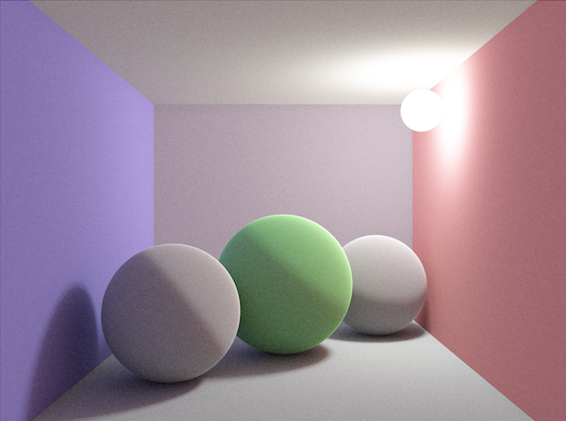
I implemented a basic prototype using WebGPU to test the algorithm. The following figure shows a screenshot of a rendering of a basic test scene.

The code for the prototype can be found here.

Introduction

Metropolis Light Transport (MLT) refers to a class of rendering algorithms which employ the Metropolis-Hastings algorithm to sample paths between light sources and a virtual camera within a virtual scene, typically in conjunction with some variant of bidirectional path tracing.

Although MLT has proved to be a very effective algorithm, it has hitherto been considered unsuitable for implementation on GPUs for several reasons:

1. The Metropolis-Hastings algorithm employs Markov chains, which, as their name implies, are sequential in nature, and not immediately amenable to parallelization.
2. Although multiple Markov chains can be utilized, each chain will be independent, and each chain will yield a shorter sequence of samples and will thus have less opportunity to converge to the targeted stationary distribution. As a result, the sampling is less effective.
3. Markov chains require the specification of an initial distribution (a first state), and if this choice is not made judiciously, it can result in startup bias, and this problem is only exacerbated by having multiple chains.
4. Some algorithms require a substantial amount of storage per Markov chain, and a multitude of chains might result in an unacceptable storage overhead.

However, there are satisfactory solutions to all of these problems:

1. It is possible to generalize the Metropolis-Hastings algorithm such that the modified algorithm is not only amenable to parallelization, but actually results in improved sampling insofar as it reduces variance and thus enjoys greater statistical efficiency.
2. The generalized version of the Metropolis-Hastings algorithm permits a single chain to be used for sampling, so there is no longer any issue with inadequate convergence.
3. It is possible to employ an initialization technique which eliminates startup bias.
4. Since there is a single chain, the overall storage is negligible.

Metropolis Light Transport

First, it is instructive to briefly review Metropolis Light Transport (MLT). The ultimate goal of the MLT rendering algorithm is to integrate the contribution of paths (from light sources to the camera) to individual pixels within an image.

\[I_j = \sum_{k=2}^N\int_{\Omega_k}h_j(\bar{x})F(\bar{x})~dV_{g_k}.\]

Here, \(\Omega_k\) is the space of all paths of length \(k\), \(N\) is the maximum path length, \(\bar{x}\) represents a path, \(h_j\) represents the pixel's support (spatial extent of the area contributing to the pixel), and \(F\) is the contribution function (ultimately, we are interested in a contribution function which is a density of radiant power over the image), and \(dV_{g_k}\) is the volume form with respect to an appropriate metric \(g_k\).

Each scene can be understood as a collection of surfaces (\(2\)-dimensional manifolds) embedded in \(\mathbb{R}^3\). Each path is modeled as a sequence \((v_1,\dots,v_k)\) of vector vertices \(v_i \in \mathbb{R}^3\). The first vertex \(v_1\) is constrained to lie on a light, the final vertex \(v_k\) is constrained to lie on the camera, and each intermediate vertex is constrained to lie on the surface of an object in the scene. The path space \(\Omega_k\) can be understood as a manifold embedded in \(\mathbb{R}^{3k}\). The metric \(g_k\) is a pullback metric induced by the Euclidean metric on the ambient manifold \(\mathbb{R}^{3k}\) (which we will describe later).

There is one such integral \(I_j\) per pixel \(j\). The goal is to estimate the value of these integrals. The Monte Carlo estimate of each integral is given by

\begin{align}I_j &= \sum_{k=2}^N \int_{\Omega_k}h_j(\bar{x})F(\bar{x})~dV_g \\&= \sum_{k=2}^N \int_{U_k}h_j(\varphi_k^{-1}(\bar{y}))F(\varphi_k^{-1}(\bar{y}))(\sqrt{\mathrm{det}g_k})~d\bar{y} \\&\approx \sum_{k=2}^N \frac{1}{n_k}\sum_{i=1}^{n_k} \frac{h_j(\varphi_k^{-1}(\bar{y}^k_i))F(\varphi_k^{-1}(\bar{y}^k_i))\sqrt{\mathrm{det}g_k}}{p_k(\varphi_k^{-1}(\bar{y}^k_i))\sqrt{\mathrm{det}g_k}} \\&= \sum_{k=2}^N \frac{1}{n_k}\sum_{i=1}^{n_k} \frac{h_j(\bar{x}^k_i)F(\bar{x}^k_i)}{p_k(\bar{x}^k_i)}\end{align}

where \(\varphi_k : \Omega_k \rightarrow U_k\) are coordinate charts and samples are chosen so that \(\varphi_k^{-1}(\bar{y}^k_i) = \bar{x}^k_i\), \(n_k\) is the number of samples used for the estimate for paths of length \(k\), \(\sqrt{\mathrm{det}g_k}\) is the square root of the determinant of the matrix representation of \(g_k\) in the coordinates induced by the chosen chart \(\varphi_k\), and each sample \(\bar{x}^k_i\) is drawn in proportion to a probability density function (PDF) \(p_k\) defined such that

\[\int_{\Omega_k}p_k(\bar{x})~dV_{g_k} = 1\]

and thus

\[\int_{U_k}p_k(\varphi^{-1}(\bar{y}))\sqrt{\mathrm{det}~g_k}~d\bar{y} = 1,\]

so the corresponding PDF on \(U_k\) is

\[p_k^*(\bar{y}) = p_k(\varphi^{-1}(\bar{y}))\sqrt{\mathrm{det}~g_k}.\]

The contribution function \(F(\bar{x})\) is typically a spectral function which means that it is computed from a density \(F(\bar{x}, \lambda)\) defined over a spectrum of wavelengths \(\lambda \in [\lambda_1, \lambda_2]\) of light.

\[F(\bar{x}) = \int_{\lambda_1}^{\lambda_2}F(\bar{x},\lambda)~d\lambda.\]

A modified Monte Carlo estimate can be used in which wavelengths \(\lambda_i\) are sampled from some distribution \(p_{\lambda}\):

\[I_j \approx \sum_{k=2}^N\frac{1}{n_k}\sum_{i=1}^{n_k} \frac{h_j(\bar{x}^k_i)F(\bar{x}^k_i, \lambda_i)}{p_k(\bar{x}^k_i)p_{\lambda}(\lambda_i)}.\]

Then, a tristimulus value (e.g., RGB or XYZ) is computed within a three-dimensional vector space called a color space using a series of matching functions \(m_i\), one for each dimension (e.g., \(m_1=m_R, m_2=m_G, m_3=m_B\)) of the color space:

\[I_j^i = \sum_{k=2}^N\int_{\Omega_k}\int_{\lambda_1}^{\lambda_2}m_i(\lambda) h_j(\bar{x})F(\bar{x}, \lambda)~d\lambda~dV_{g_k}.\]

Thus, at each pixel, a vector of values (e.g., \(\langle I_j^1,I_j^2,I_j^3\rangle = \langle R, G, B \rangle\)) within a color space is ultimately computed. However, Metropolis sampling requires a scalar function. The solution used in MLT is to designate a scalar contribution function which is a scalar function which represents \(F(\bar{x})\) and is, in some sense, proportional to \(F(\bar{x})\). The usual choice is the photometric quantity known as luminance \(Y\) defined in terms of a spectral response function \(V\) as follows:

\[Y(\bar{x}) = \int_{\lambda_1}^{\lambda_2}V(\lambda)F(\bar{x}, \lambda)~d\lambda.\]

In terms of a linear RGB color space, the luminance is simply:

\[Y = 0.2126 \cdot R + 0.7152 \cdot G + 0.0722 \cdot B.\]

The goal is to generate a sequence of samples of paths of length \(k\) proportional to the PDF \(p_k\) corresponding to the scalar contribution function, defined as follows:

\[p_k(\bar{x}) = \frac{Y(\bar{x})}{\int_{\Omega_k}Y(\bar{x})~dV_{g_k}}.\]

Thus, paths will be sampled in a manner proportional to their luminance (roughly, their brightness). The Metropolis-Hastings algorithm devises a Markov chain whose stationary distribution is equal to \(p_k\). The pixel measurement can then be estimated using the Monte Carlo estimator (neglecting the spectral terms) as

\begin{align}I_j &\approx \sum_{k=2}^N \frac{1}{n_k}\sum_{i=1}^{n_k} \frac{h_j(\bar{x})F(\bar{x}_i)}{p_k(\bar{x}_i)} \\&= \sum_{k=2}^N\frac{1}{n_k}\sum_{i=1}^{n_k} \frac{h_j(\bar{x})F(\bar{x}_i)}{\frac{Y(\bar{x})}{\int_{\Omega_k}Y(\bar{x})~dV_{g_k}}} \\&= \sum_{k=2}^N\frac{1}{n_k}\sum_{i=1}^{n_k}\frac{h_j(\bar{x})F(\bar{x})}{Y(\bar{x}_i)} \cdot \left(\int_{\Omega_k}Y(\bar{x})~dV_{g_k}\right) \\&= \sum_{k=2}^N\frac{b_k}{n_k}\sum_{i=1}^{n_k}\frac{h_j(\bar{x})F(\bar{x})}{Y(\bar{x}_i)},\end{align}

where \(b_k = \int_{\Omega_k}Y(\bar{x})~dV_{g_k}\). The quantities \(b_k\) can be estimated in an initialization phase using a Monte Carlo estimator with a uniform probability distribution and a fixed number of samples.

Primary Sample Space Metropolis Light Transport

The original MLT algorithm employed a set of specialized path mutation rules directly within path space which are challenging to implement properly and non-symmetric. The Primary Sample Space Metropolis Light Transport (PSSMLT) algorithm instead performs path mutations in the primary sample space, i.e., the space \(\mathcal{U}_k = (0,1)^{d(k)}\) of vectors of uniformly-distributed random numbers in the range \((0,1)\) used to generate paths (where \(d(k)\) indicates the number of random numbers needed for paths of length \(k\)). Thus, the path space manifold \(\Omega_k\) is a \(d(k)\)-dimensional manifold. The metric \(g_k\) can be seen as the pullback metric \(S_k^*g\) of the Euclidean metric \(g\) on \(\mathbb{R}^{3k}\).

Let \(S_k\) denote the mapping from primary sample space \(\mathcal{U}^k\) to path space \(\Omega_k\). We can treat \(S_k^{-1}\) as a coordinate chart since \((0,1)^{d(k)}\) is an open subset of \(\mathbb{R}^{d(k)}\). This implicitly makes the following assumptions: each vector of numbers generates a unique path, each path corresponds to a unique vector of numbers, thus there is a bijection, and this mapping is smooth. These assumptions will not be true in general, but there are various technical workarounds; the final Monte Carlo estimate remains the same. We then compute the integral with respect to the volume form as follows:

\begin{align}\sum_{k=2}^N\int_{\Omega_k}Y(\bar{y})~dV_{g_k} &= \int_{\mathcal{U}_k}Y(S_k(\bar{x}))\sqrt{\mathrm{det}~ g_k}~d\bar{x}.\end{align}

For open scenes, we can posit a hypothetical surface that encloses the entire scene, such that any path intersecting this enclosure has a contribution of \(0\); this way every vector of random numbers corresponds to a path, i.e., those that generate invalid paths that escape the scene can be considered "paths" for theoretical purposes. Likewise, whenever subpaths cannot be connected (e.g., due to an intervening surface obstructing the connection), we can consider them "paths" yet ensure that their contribution is \(0\).

Thus, we define a modified scalar contribution function \(Y^*\) as

\[Y^*(\bar{x}) = Y(S_k(\bar{x}))(\sqrt{\mathrm{det}~g_k}).\]

However, we do not actually need to compute the term \(\sqrt{\mathrm{det}~g}\) directly. The same pullback applies to any probability density function (PDF) \(p\) on path space so that the corresponding PDF \(p^*\) in primary sample space is

\[p_k^*(\bar{x}) = p_k(S_k(\bar{x}))\sqrt{\mathrm{det}~g_k}\]

and, since the probability density function \(p^*\) for a uniformly distributed random variable over the domain \(\mathcal{U}=(0,1)^{d(k)}\) is constant, i.e., \(p_k^*(\bar{x})=1\), it follows that

\[\sqrt{\mathrm{det}~{g_k}} = \frac{1}{p_k(S_k(\bar{x}))},\]

and hence

\[Y^*(\bar{x}) = \frac{Y(S_k(\bar{x}))}{p_k(S_k(\bar{x}))}.\]

The Metropolis-Hastings algorithm is then applied to produce samples used for a Monte Carlo estimate of this integral. The target distribution \(\pi\) is the scalar contribution function's own distribution:

\[\pi_k(\bar{x}) = \frac{Y^*(\bar{x})}{\int_{\mathcal{U}_k}Y^*(\bar{x})~d\bar{x}}.\]

PSSMLT proposes each new primary sample by mutating the current primary sample. PSSMLT uses two types of mutations on primary samples:

• A large step mutation which replaces the entire vector of random numbers with a new vector
• A small step mutation which applies small perturbations to each of the random numbers.

Since each of these mutations is symmetric, the proposal distribution is symmetric, and thus the acceptance distribution simplifies to

\begin{align}A(\bar{x}_i \mid \bar{x}_j) &= \mathrm{min}\left(1, \frac{\pi_k(\bar{x}_j)}{\pi_k(\bar{x}_i)}\right) \\&= \mathrm{min}\left(1, \frac{Y^*(\bar{x}_j)}{Y^*(\bar{x}_i)}\right).\end{align}

Multiplexed Metropolis Light Transport

The Multiplexed Metropolis Light Transport (MMLT) algorithm modifies the PSSMLT in the following ways:

• Only a single bidirectional path tracing (BDPT) connection strategy is used. Typically, in bidirectional path tracing, once a path is constructed, all possible subpaths are constructed and used.
• This connection strategy is determined by a random number which is a component of the primary sample vector.
• A set of Markov chains are maintained in parallel, one for each path length; it is in this sense "multiplexed".

The MMLT algorithm is more amenable to implementation on the GPU since processing a single BDPT connection requires the storage of much less state whereas processing all BDPT sub-path connections would require the maintenance of a substantial amount of state in memory.

We can now describe the overall MMLT algorithm.

First, for each path length \(k\), \(n\) uniformly random primary samples \(\bar{x}_i\) are generated and a Monte Carlo estimate is computed, which simplifies to the following since the PDF used for sampling is uniform (constant \(p(\bar{x}) = 1\)):

\[b_k = \int_{\mathcal{U}_k}Y^*(\bar{x}_i)~d\bar{x} \approx \frac{1}{n_k}\sum_{i=1}^{n_k} Y^*(\bar{x}_i).\]

An initial primary sample \(\bar{x}_{\text{current}}\) is selected, for instance, by constructing a PDF from each of the scalar contributions of each of the paths used in the initialization phase and then sampling this PDF.

Then, the Metropolis-Hasting algorithm is used to generate samples proportional to the PDF of the scalar contribution function \(Y^*\) and these samples are used to compute a Monte Carlo estimate for the measurement equation.

1. Sample a path length \(k\) in proportion to the distribution computed in the initialization phase.
2. Generate a uniform random number to determine the mutation strategy (small step vs. large step) according to a configurable probability \(s\) for small step and \(1-s\) for large step. If \(r < s\), then a small step is used; otherwise, a large step is used.
3. Generate a proposal primary sample \(\bar{x}_{\text{proposal}}\) from the current primary sample \(\bar{x}_{\text{current}}\) using the selected mutation strategy.
4. Generate a path \(S(\bar{x}_{\text{proposal}})\) using the proposed primary sample.
5. Compute the acceptance probability \(a = \mathrm{min}\left(1, \frac{Y^*(\bar{x}_{\text{proposal}})}{Y^*(\bar{x}_{\text{current}})}\right)\).
6. Generate a uniform random number \(r\) in the range \((0,1)\). If \(r < a\), accept the proposal (set \(\bar{x}_{\text{current}} = \bar{x}_{\text{proposal}}\)). Otherwise, reject the proposal (do not update \(\bar{x}_{\text{current}}\)).
7. Add both the current and proposal contributions to the image, weighting each by \(1-a\) and \(a\), respectively.
8. Repeat to step 1.

Generalized Metropolis-Hastings

The primary impediment to parallelization is the fact that the Metropolis-Hastings algorithm generates a single proposal at a time. However, it is possible to generalize the Metropolis-Hastings algorithm in order to permit multiple proposals. Thus, we can generate one proposal per path and generate many paths in parallel, for instance. This generalized variant is described in detail in the following post:

Parallel Metropolis Hastings

The end result is a modification to the acceptance distribution; for current state \(\bar{x}_i\) and \(N\) proposal states \(\bar{x}_j\), the acceptance distribution becomes

\[A(\bar{x}_i, \bar{x}_j) = \begin{cases}\frac{1}{N}\mathrm{min}\left(1,\frac{Y^*(\bar{x}_j)}{Y^*(\bar{x}_i)}\right) & \text{if}~i \ne j \\ 1 - \sum_{k \ne i}A(\bar{x}_i,\bar{x}_k) & \text{if}~i = j.\end{cases}\]

Then, to determine whether to accept or reject, we sample from \(A_i = A(\bar{x}_i,\cdot)\) (e.g., by computing its cumulative distribution function (CDF) \(F_{A_i}\), generating a uniformly distributed random number \(r \in (0,1)\), and then selecting the least index \(j\) such that \(r < F_{A_i}(\bar{x}_j)\)).

The PMLT Algorithm

We now give a high-level overview of the PMLT algorithm.

1. Phase 1. For each path length \(k\):
   1. Generate \(n\) paths \(\bar{x}_i\) of length \(k\) in parallel using BDPT, computing their scalar contribution \(Y^*(\bar{x}_i)\).
   2. Compute the Monte Carlo estimate of the scalar contribution integral \(b_k = \frac{1}{n}\sum_{i=1}^n Y^*(\bar{x}_i)\).
   3. Construct a PDF of the scalar contributions per path: \(p(\bar{x}_i) = Y^*(\bar{x}_i)/\sum_{j=1}^nY^*(\bar{x}_j)\) and a corresponding CDF \(F\) (as a prefix sum).
   4. Sample this PDF by generating a uniformly-distributed random number \(r \in (0,1)\) and selecting the least index \(j\) such that \(r < F(\bar{x}_j)\), e.g., by using a binary search. Initialize the current state for path length \(k\) to the primary sample (vector of random numbers) used to generate path \(j\). These numbers need not be stored anywhere - they can be computed (see the section on pseudo-random number generation). Since counter-based PRNGs are used, it is only necessary to compute the indices that path \(j\) used during initialization. This primary sample is stored in the state associated with the respective chain (there is one Markov chain per path length \(k\)).
2. For each path, determine its length during the primary rendering phase as follows. Assign each a path length \(k\) in proportion to the distribution determined by the discrete PDF \(p(k) = b_k/\sum_k b_k\). There should be (modulo rounding) \(N_k = p(k) \cdot n\) paths of length \(k\). The number of paths of length \(k\) is thus in proportion to the overall scalar contribution of paths of length \(k\) during the initialization phase.
3. Phase 2. Generate \(n\) proposal paths in parallel using bidirectional path tracing. Each path will be of the length assigned to it in the initialization phase. There will be \(N_k\) paths of length \(k\). For a configurable small-step probability \(p_{\text{small}}\), a total of \(p_{\text{small}} \cdot N_k\) paths should be proposed using small-step mutations and a total of \((1-p_{\text{small}}) \cdot N_k\) paths should be proposed using large-step mutations.
4. Compute the acceptance distributions \(A_k(\bar{x}_i,\cdot)\) for each path length \(k\). \[A_k(\bar{x}_i, \bar{x}_j) = \begin{cases}\frac{1}{N_k}\mathrm{min}\left(1,\frac{Y^*(\bar{x}_j)}{Y^*(\bar{x}_i)}\right) & \text{if}~i \ne j \\ 1 - \sum_{l \ne i}A_k(\bar{x}_i,\bar{x}_l) & \text{if}~i = j.\end{cases}.\]
5. Contribute the contributions of each path to their respective pixel (or pixels, if using convolution filters), weighting each using \(A_k(\bar{x}_i, \bar{x}_j)\) as a weight.
6. Apply generalized Metropolis-Hastings: sample each \(A_k(\bar{x}_i,\cdot)\) using its corresponding CDF and then update the current state (primary sample vector) for each respective chain corresponding to path length \(k\) by computing the primary sample used to generate the sampled path (again, only the index needs to be recomputed, the random numbers used for each path are not stored anywhere). Continue to step 3.
7. Finally: note that each iteration produces exactly one Monte Carlo sample per chain irrespective of the the number of proposals per chain, that is, the weighted sum of the contributions due to each proposal multiplied by the respective weights \(A_k(\bar{x}_i, \bar{x}_j)\) for each proposal counts as a single Monte Carlo sample, so that each of the \(n_k\) (where \(n_k\) is the total number of Monte Carlo samples for paths of length \(k\)) are equal to \(N_I\), and the final Monte Carlo estimate should be scaled by a factor of \(1/N_I\), where \(N_I\) is the number of iterations. The estimate is "Rao-Blackwellized" (see the discussion in this post).

Technical Challenges

There are several significant technical challenges which implementations must face, including the following:

• Generation of pseudo-random numbers, and the memory-efficient representation of primary samples (vectors of random numbers),
• Computation of multiple importance sampling (MIS) weights,
• Constructing PDFs and CDFs efficiently and sampling them efficiently,
• Updating the image (since distinct paths can correspond to the same pixel(s) which can result in race conditions when updating the image raster),
• Handling queueing efficiently and in a thread-safe manner (since many threads will be updating the same queue concurrently).

Pseudo-Random Numbers

Most rendering algorithms are stochastic in nature and require pseudo-random number generators (PRNGs). However, most PRNGs require the maintenance of some sort of state, which makes most of them inherently sequential in nature since this state is typically updated in a serial fashion. This means that many PRNGs are not appropriate for use with GPUs. However, there is a class of PRNGs called counter-based random number generators (CBRNGs) which consists of PRNGs that do not rely on state but rather produce numbers based on an integer parameter which represents the index of the number within the generated sequence of numbers. Thus, the numbers may be generated in any order, and CBRNGs are appropriate for use with GPUs.

In the post "Counter-Based Pseudo-Random Number Generators on the GPU", I described the theory and implementation of a particular algorithm called the Squares CBRNG. Using this algorithm, it is possible to generate pseudo-random numbers on the GPU.

However, since many numbers will be requested in parallel, it is necessary to establish a scheme for partitioning the sequence of random numbers into multiple subsequences and to dedicate the subsequences for various purposes so that the same indices are not used for distinct purposes. I will begin by describing an example of a hierarchical partitioning scheme.

The algorithm traces paths in parallel. In my experiment, I generated 1 million paths, for instance. Each path is comprised of multiple vertices. Random numbers are always requested when processing a vertex (for instance, when sampling a reflectance function at an intersection point in order to determine the next direction to trace). Thus, it is possible to establish an upper bound \(v\) on the number of random numbers required by each vertex (for instance, in my experimental implementation, \(4\) numbers or less are required at each vertex). Then, for a path of length \(n\), at most \(n \cdot v\) numbers are required.

However, the situation is slightly more subtle than this due to certain details of the particular algorithm employed. As described previously, the PMLT algorithm is based on the Multiplexed Metropolis Light Transport (MMLT) algorithm which is based on the Primary Sample Space Metropolis Light Transport (PSSMLT) algorithm. Such algorithms maintain a vector of random numbers (called a primary sample) which is used as a proxy for a path (since each such vector uniquely determines a particular path). Paths can then be mutated by mutating the primary sample, which is generally much simpler than mutating the path itself. The MMLT algorithm additionally specifies an extra component of this primary sample vector which determines the particular bidirectional path tracing strategy to use (for instance, whether, for a path of length \(5\), to trace \(3\) vertices from the camera and \(2\) from the light, or to trace \(1\) from the camera and \(4\) from the light, etc.). Thus, each strategy is a tuple \((c, l)\) consisting of the number of camera vertices and the number of light vertices. To prevent interference when the strategy is updated, the random numbers for camera and light subpaths are kept separate (so that, for instance, a number which was previous used at a camera vertex is not accidentally repurposed for use at a light vertex, etc.). Each strategy can allocate at most \(n \cdot v\) numbers to each subpath. Thus, for a path of length \(n\), there are \(2 \cdot n \cdot v + 1\) numbers, \(n \cdot v\) for each subpath, and \(1\) for the strategy.

Each chain contains an array of (at least) \(2 \cdot n \cdot v + 1\) random numbers representing the current primary sample for the chain. Each chain uses a distinct PRNG since the random numbers generated by each chain are independent (the Squares32 CBRNG requires a key and an index, so each chain uses a distinct key).

To request a random number, the index of the random number must be computed (for Squares32, the index ranges from \(0\) to \(2^{64}-1\)). This affords a powerful technique: we only need to store one primary sample per chain, which amounts to a negligible amount of overall storage. We do not need to store anything per path since we can devise a formula for computing the indices for each random number requested within a path. During each rendering iteration, each path will propose a mutation of the primary sample, which will either be a large step mutation or a small step mutation. Since each proposal is a function of the current sample (stored within the chain) and the indices used by the path, it can be computed and does not need to be stored. The following pseudocode illustrates the idea.

let index = iteration * numbers_per_iteration + path_index * numbers_per_path + number_offset;
let random_number = squares32(index, key);
if step_type == LARGE_STEP {
  return random_number;
} else {
  let current_number = numbers[number_offset];
  return perturb(current_number, random_number);
}

In this pseudocode listing, the following definitions are used:

• path_index is the index of the path relative to the chain; this index is computed during initialization. For each path length \(k\), there is precisely one chain and \(n_k\) paths. The indices range from \(0\) to \(n_k-1\) and are assigned arbitrarily (paths will be stored in an SOA format and the path_index is the index within the respective arrays).
• numbers_per_path is the maximum numbers required per path (computed as a function of the path length and numbers per vertex, etc., as \(k \cdot v + 1\)).
• number_offset is the index of the random number being requested. Each path is allocated a "stream" of numbers_per_path numbers.
• iteration is the index of the rendering iteration (each iteration consists of fully processing all paths once).
• numbers_per_iteration is a pre-computed value which represents the count of random numbers required per iteration.
• key represents the CBRNG key used for the respective chain.
• step_type is the mutation type assigned to the respective path (small or large step).
• numbers represents the primary sample, i.e., the vector of numbers assigned to the respective chain.
• squares32 is the Squares32 CBRNG.
• perturb represents a random perturbation of a number.

The following WGSL code shows this calculation concretely:

fn rand(chain_id: u32, global_path_index: u32, number_offset: u32) -> f32 {
    let offset = path.index[global_path_index] * chain.numbers_per_path[chain_id] + number_offset;
    let iteration_offset = u64_mul(u64_from(chain.iteration[chain_id]), u64_from(chain.numbers_per_iteration[chain_id]));
    let index = u64_add(iteration_offset, u64_from(offset));
    let key = U64(chain.key[HI][chain_id], chain.key[LO][chain_id]);
    let random_number = squares32(index, key);
    if  path.step_type[global_path_index] == LARGE_STEP {
        return random_number;
    } else {
        let value = chain.numbers[number_offset][chain_id];
        let perturbation = SIGMA
          * sqrt(2.0) 
          * erf_inv(2.0 * random_number - 1.0);
        let result = value + perturbation;
        return result - floor(result);
    }
}

fn populate_random_numbers(chain_id: u32, global_path_index: u32) {
  for (var i: u32 = 0; i < chain.numbers_per_path[chain_id]; i++) {
    chain.numbers[i][chain_id] = rand(chain_id, global_path_index, i);
  }
}

Then, a convention needs to be established for ensuring a consistent assignment of values for number_offset. The convention used in the experiment is that camera vertices are stored first, light vertices are stored next, and the technique state (number that determines the BDPT connection strategy) is stored last. The index of the vertex within the path is stored as part of the path state. The number_offset can be computed using this state.

Once a particular proposal is selected via the generalized Metropolis-Hastings acceptance distribution, the chain's current proposal can be updated (see the populate_random_number function in the listing above). This proposal is not stored anywhere, but is rather re-computed using the appropriate parameters.

Thus, CBRNGs obviate the need to store the proposed primary samples.

Multiple Importance Sampling

Metropolis Light Transport employs multiple importance sampling using the balance heuristic to compute a weight for each path contribution. Computing MIS weights is straightforward on a CPU implementation in which all vertices in a path can be examined together. However, on the GPU, the path is constructed incrementally one vertex at a time and prior vertices are not stored. MIS is a global property involving all vertices. However, on the GPU, vertices are only inspected locally. This presents a challenge when computing the MIS weights on a GPU.

With bidirectional path tracing (BDPT), two independent paths are traced: one starting at the camera, and one starting at the light. Then, each subpath is connected resulting in a complete path from light to camera.

With BDPT, light subpath \(q_0,\dots,q_{s-1}\) consisting of \(s\) vertices is constructed incrementally, starting with a point \(q_0\) on a light, and a camera subpath \(p_0,\dots,p_{t-1}\) is constructed incrementally, starting with a point \(p_0\) on the camera, resulting in a composite path proceeding from the light to the camera:

\[\bar{p} = q_0,\dots,q_{s-1},p_0,\dots,p_{t-1}.\]

The specification \((s,t)\) of the number of light and camera vertices is called a strategy or a technique. For strategies with \(t \ge 2\), at the point \(p_0\) (which, on a pinhole camera is a fixed point), a direction is sampled which proceeds from this point through the image plane, thus designating a particular pixel. The next vertex \(p_1\) is found by computing the closest intersection along this direction, if any. Likewise, a point \(q_0\) is sampled on the light and then a direction is sampled and an intersection is performed to compute the next vertex \(q_1\), etc. Finally, a connection is performed between vertices \(p_{t-1}\) and \(q_{s-1}\); these vertices are connectable if they are mutually visible (a ray can be cast between them without being occluded). However, the path throughput might be \(0\) if the BSDFs at the vertices do not scatter light in the respective direction (e.g. a connection containing a vertex on a perfect specular surface is unlikely to succeed since it is unlikely that the connection coincides with the reflection direction).

Multiple importance sampling (MIS) is used to compute a probability density function (PDF) for path construction. The balance heuristic is used to weight path contributions. In order to employ this heuristic, the probability densities for all hypothetical path constructions must be known. The following depicts an actual strategy and all other hypothetical strategies.

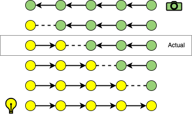
We can denote a path \(\bar{x}\) of length \(n\) constructed with strategy \((s,t)\) (where \(s + t = n\)), from camera subpath \(p_o,\dots,p_{t-1}\) and light subpath \(q_0,\dots,q_{s-1}\) as

\[\bar{x} = x_0,\dots,x_{n-1} = q_0,\dots,q_{s-1},p_0,\dots,p_{t-1}.\]

Each vertex is denoted \(x_i\) for \(0 \leq i \lt n\). Note that the PDFs for vertices are computed with respect to area (they are PDFs per unit area). The expression \(p^{\rightarrow}(x_i)\) represents the PDF per unit area of sampling vertex \(x_i\) along a light subpath. The expression \(p^{\leftarrow}(x_i)\) represents the PDF per unit area of sampling vertex \(x_i\) along a camera subpath. These will generally differ since they will involve conversions from solid angle densities of different BRDFs, etc. The path density for the actual strategy \((s,t)\) is denoted \(p_s(\bar{x})\) (where implicitly \(t = n - s\)) and is given by

\begin{align}p_s(\bar{x}) &= p^{\rightarrow}(q_0),\dots,p^{\rightarrow}(q_{s-1}),p^{\leftarrow}(p_{t-1}),\dots,p^{\leftarrow}(p_0) \\&= p^{\rightarrow}(x_0),\dots,p^{\rightarrow}(x_{s-1}),p^{\leftarrow}(x_s),\dots,p^{\leftarrow}(x_{n-1}).\end{align}

For a given actual strategy \((s,t)\) used to construct a given path, we want to consider each hypothetical strategy \((i,j)\) which could have been used to construct the same path. Thus, it must be the case that \(i+j = s+t\) in order to preserve path length. We denote the path density of a hypothetical path construction with strategy \((i,j)\) on path \(\bar{x}\) as \(p_i(\bar{x})\), where implicitly \(j = n - i\):

\[p_i(\bar{x}) = p^{\rightarrow}(x_0),\dots,p^{\rightarrow}(x_{i-1}),p^{\leftarrow}(x_i),\dots,p^{\leftarrow}(x_{n-1}).\]

To compute the MIS weight \(w_s(\bar{x})\) for an actual strategy \(s\), we must compute

\[w_s = \frac{p_s(\bar{x})}{\sum_{i=1}^np_i(\bar{x})}.\]

There is an efficient and more numerically stable way to compute the MIS weight which I learned from PBRT. However, this approach computes values in the reverse order that they are encountered during GPU rendering, so I had to modify it to compute values in a different order.

First, divide both numerator and denominator of \(w_s(\bar{x})\) by \(p_s(\bar{x})\) to obtain the equivalent expression

\[w_s = \frac{1}{\sum_{i=1}^n\frac{p_i(\bar{x})}{p_s(\bar{x})}}.\]

Next, split this expression as follows (noting that \(p_i(\bar{x}) = p_s(\bar{x}\) when \(i = s\)):

\[w_s = \left(\sum_{i=1}^{s-1}\frac{p_i(\bar{x})}{p_s(\bar{x})} + 1 + \sum_{i=s+1}^{n}\frac{p_i(\bar{x})}{p_s(\bar{x})} \right)^{-1}.\]

Denote the ratios therein as follows:

\[r_i(\bar{x}) = \frac{p_i(\bar{x})}{p_s(\bar{x})}.\]

These ratios can also be expressed as follows:

\[r_i(\bar{x}) = \begin{cases}\frac{p_i(\bar{x})}{p_{i+1}(\bar{x})}\frac{p_{i+1}(\bar{x})}{p_s(\bar{x})} = \frac{p_i(\bar{x})}{p_{i+1}(\bar{x})}r_{i+1}(\bar{x}) = \prod_{j=i}^{s-1}\frac{p_j(\bar{x})}{p_{j+1}(\bar{x})} & (i \lt s), \\ 1 & (i = s), \\ \frac{p_i(\bar{x})}{p_{i-1}(\bar{x})}\frac{p_{i-1}(\bar{x})}{p_s(\bar{x})} = \frac{p_i(\bar{x})}{p_{i-1}(\bar{x})}r_{i-1}(\bar{x}) = \prod_{j=s+1}^i\frac{p_j(\bar{x})}{p_{j-1}(\bar{x})} & (i \gt s).\end{cases}\]

The ratios between path densities of strategies that differ by \(1\) share all terms except for one:

\[\frac{p_i(\bar{x})}{p_{i+1}(\bar{x})} = \frac{p^{\rightarrow}(x_0)\dots p^{\rightarrow}(x_{i-1})p^{\leftarrow}(x_i)p^{\leftarrow}(x_{i+1})\dots p^{\leftarrow}(x_{n-1})}{p^{\rightarrow}(x_0)\dots p^{\rightarrow}(x_{i-1})p^{\rightarrow}(x_i)p^{\leftarrow}(x_{i+1})\dots p^{\leftarrow}(x_{n-1})} = \frac{p^{\leftarrow}(x_i)}{p^{\rightarrow}(x_i)},\]

\[\frac{p_i(\bar{x})}{p_{i-1}(\bar{x})} = \frac{p^{\rightarrow}(x_0)\dots p^{\rightarrow}(x_{i-2})p^{\rightarrow}(x_{i-1})p^{\leftarrow}(x_i) \dots p^{\leftarrow}(x_{n-1})}{p^{\rightarrow}(x_0)\dots p^{\rightarrow}(x_{i-2})p^{\leftarrow}(x_{i-1})p^{\leftarrow}(x_i) \dots p^{\leftarrow}(x_{n-1})} = \frac{p^{\rightarrow}(x_{i-1})}{p^{\leftarrow}(x_{i-1})}.\]

Thus, we can rewrite the expression for each ratio as

\[r_i(\bar{x}) = \begin{cases}\frac{p_i(\bar{x})}{p_{i+1}(\bar{x})}\frac{p_{i+1}(\bar{x})}{p_s(\bar{x})} = \frac{p^{\leftarrow}(x_i)}{p^{\rightarrow}(x_i)}r_{i+1}(\bar{x}) = \prod_{j=i}^{s-1}\frac{p^{\leftarrow}(x_j)}{p^{\rightarrow}(x_j)} & (i \lt s), \\ 1 & (i = s), \\ \frac{p_i(\bar{x})}{p_{i-1}(\bar{x})}\frac{p_{i-1}(\bar{x})}{p_s(\bar{x})} = \frac{p^{\rightarrow}(x_{i-1})}{p^{\leftarrow}(x_{i-1})}r_{i-1}(\bar{x}) = \prod_{j=s+1}^i\frac{p^{\rightarrow}(x_{j-1})}{p^{\leftarrow}(x_{j-1})} & (i \gt s).\end{cases}\]

We use the following abbreviations:

\[R^L_i(\bar{x}) = \frac{p^{\leftarrow}(x_i)}{p^{\rightarrow}(x_i)},\]

\[R^C_i(\bar{x}) = \frac{p^{\rightarrow}(x_{i-1})}{p^{\leftarrow}(x_{i-1})}.\]

Thus, we can rewrite the expression for each ratio as

\[r_i(\bar{x}) = \begin{cases}\prod_{j=i}^{s-1}R^L_i(\bar{x}) & (i \lt s), \\ 1 & (i = s), \\ \prod_{j=s+1}^i R^C_i(\bar{x}) & (i \gt s).\end{cases}\]

Next, observe that

\[\prod_{j=i}^{s-1}R^L_j(\bar{x}) = \left(\prod_{j=1}^{i-1} \frac{1}{R^L_j(\bar{x})}\right)\left(\prod_{k=1}^{s-1}R^L_k(\bar{x})\right)\]

and

\[\prod_{j=s+1}^i R^C_j(\bar{x}) = \left(\prod_{j=i+1}^n \frac{1}{R^C_j(\bar{x})}\right)\left(\prod_{k=s+1}^nR^C_k(\bar{x})\right).\]

It then follows that

\[\sum_{i=1}^{s-1}r_i(\bar{x}) = \left(\prod_{k=1}^{s-1}R^L_k(\bar{x})\right)\left(\left(\sum_{i=1}^{s-1}\prod_{j=1}^{i-1} \frac{1}{R^L_j(\bar{x})}\right) + 1\right)\]

and

\[\sum_{i=s+1}^n r_i(\bar{x}) = \left(\prod_{k=s+1}^nR^C_k(\bar{x})\right)\left(\left(\sum_{i=s+1}^n\prod_{j=i+1}^n \frac{1}{R^C_j(\bar{x})}\right) + 1\right).\]

When constructing a light path, the index \(i\) will proceed from \(1\) to \(s-1\); thus, the sum of products can be computed in order. When constructing a camera path, the index \(i\) will proceed from \(n\) to \(s+1\); thus, the sum of products can be computed in order.

If we number the vertices as follows (so that the camera vertices are ordered according to the order in which they are constructed and not according to their order within the path)

\[\bar{p} = q_0,\dots,q_{s-1},p_{t-1},\dots,p_0\]

then the expression becomes

\[\sum_{i=1}^{t-1}r_i(\bar{x}) = \left(\prod_{k=1}^{t-1}R^C_k(\bar{x})\right)\left(\left(\sum_{i=1}^{t-1}\prod_{j=1}^{i-1} \frac{1}{R^C_j(\bar{x})}\right) + 1\right)\]

which has the same form as the expression involving \(R^L\).

Finally, if we define \(p_{\text{fwd}} = p^{\rightarrow}\) and \(p_{\text{rev}} = p^{\leftarrow}\) for light sub-paths and \(p_{\text{fwd}} = p^{\leftarrow}\) and \(p_{\text{rev}} = p^{\rightarrow}\) for camera sub-paths, then we can utilize a single ratio \(R\) defined as

\[R_i(\bar{x}) = \frac{p_{\text{rev}}(\bar{x}_i)}{p_{\text{fwd}}(\bar{x}_i)}\]

and a single expression (where \(N = s\) or \(N = t\)):

\[\sum_{i=1}^{N-1}r_i(\bar{x}) = \left(\prod_{k=1}^{N-1}R_k(\bar{x})\right)\left(\left(\sum_{i=1}^{N-1}\prod_{j=1}^{i-1} \frac{1}{R_j(\bar{x})}\right) + 1\right).\]

Thus, the calculation is symmetric in camera and light sub-paths; the forward and reverse PDF evaluations just need to be maintained accordingly, but the same computations can be used for both sub-paths otherwise.

This expression permits us to accumulate the MIS weights one vertex at a time and does not require storing an inordinate amount of state. To compute the MIS weight one vertex at a time, only the following data is required:

• the forward and reverse PDF evaluations (the forward is cached, the reverse can be computed),
• the sum \(\sum_{i=1}^{N-1}\prod_{j=1}^{i-1} \frac{1}{R_j(\bar{x})}\), accumulated incrementally,
• the product \(\prod_{k=1}^{t-1}R_k(\bar{x})\), accumulated incrementally.

Thus, for example, given sum of products

\[n_1 + n_2n_2 + n_1n_2n_3 + n_1n_2n_3n_4,\]

we can reverse the order of the products by computing

\[\left(\frac{1}{n_1} + \frac{1}{n_1n_2} + \frac{1}{n_1n_2n_3}\right) \cdot n_1n_2n_3n_4 + n_1n_2n_3n_4 = n_4 + n_4n_3 + n_4n_3n_2 + n_4n_3n_2n_1.\]

We can also compute

\[\left(\frac{1}{n_1} + \frac{1}{n_1n_2} + \frac{1}{n_1n_2n_3} + \frac{1}{n_1n_2n_3n_4}\right) \cdot n_1n_2n_3n_4 - 1 + n_1n_2n_3n_4 = n_4 + n_4n_3 + n_4n_3n_2 + n_4n_3n_2n_1,\]

which, for implementation-specific reasons, is what the prototype actually does.

fn get_mis_weight(i: u32) -> f32 {
    let sum_ri = path.sum_inv_ri[CAMERA][i] * path.prod_ri[CAMERA][i] + path.prod_ri[CAMERA][i] - 1.0 
        + path.sum_inv_ri[LIGHT][i] * path.prod_ri[LIGHT][i] + path.prod_ri[LIGHT][i] - 1.0;
    return 1.0 / (1.0 + sum_ri);
}

Start-up Bias Elimination

Each Markov chain must begin in an initial state. The Metropolis-Hastings algorithm assumes that the initial state was sample in proportion to the target distribution. If this is not the case, start-up bias can occur. However, there are techniques for eliminating start-up bias.

See the discussion in the PBRT book about start-up bias elimination.  The idea is to generate a set of \(n\) candidate samples \(\bar{x}_i\) that are candidates for the initial state. In the PMLT algorithm, this is done in the initialization phase. In the PMLT algorithm, a starting sample is chosen by sampling the distribution according to the PDF

\[p(\bar{x}_i) = \frac{Y^*(\bar{x}_i)}{\sum_{i=1}^nY^*(\bar{x}_i)}.\]

WebGPU Prototype

A prototypical implementation in WebGPU was developed as a basic proof of concept. The code is available here.

WebGPU

WebGPU, as the name implies, is indeed a GPU interface, with a Javascript specification, which permits web browsers to interface with GPUs. It is a W3C standard in development. However, it is much more than simply a browser interface: it is a general-purpose interface which abstracts away from various frameworks such as DirectX, Metal, and Vulkan. Thus, it is possible to develop one portable implementation in WebGPU versus multiple implementations in various other interfaces. It has implementations in other programming languages (e.g. wgpu for Rust) and can be used outside the context of a browser.

Efficiency

Designing programs which utilize the resources of a GPU efficiently is challenging. In general, designs aim for the following features:

• Reduced CPU to GPU coordination. Transferring buffered data from the GPU to the CPU can cause significant bottlenecks. Thus, it is generally desirable to avoid the requirement to read results from kernel launches back to the CPU in order to determine how to proceed.
• Minimal thread divergence. GPU threads are grouped into groups, sometimes called "warps", which execute the same instruction at the same time, yet on different data (SIMD - single instruction, multiple data). If threads within a group diverge, i.e., require execution of different instructions, then the group must be partitioned into sub-groups, one per instruction, and each sub-group then executes serially. Thus, it is desirable to avoid conditional logic (in general, but not always).
• Locality of memory access. Threads within thread groups should ideally access nearby memory locations, permitting pre-fetching of memory, etc.
• Utilization. Threads should be kept busy doing work continually.

The prototype attempts to apply these principles, favoring some over others.

Reduced Coordination

The implementation is designed so that kernels are dispatched in a mostly static manner so that results from GPU kernel dispatches don't have to be read back to the CPU in order to determine which subsequent kernels to dispatch. This also means that large buffers of commands can be submitted together all at once.

The code makes ample use of WebGPU's support for indirect dispatch, which permits the number of workgroups dispatched to be read from memory updated by the kernels (rather than being specified at the CPU).

Divergence

The code attempts to avoid thread divergence. For instance, instead of

if valid {
  queue_id = CONTRIBUTE_QUEUE_ID;  
} else {
  queue_id = NULL_QUEUE_ID;
}

the following is used

queue_id = choose_u32(valid, CONTRIBUTE_QUEUE_ID, NULL_QUEUE_ID);

where choose_u32 is a utility function (there is also a similar select function built into WGSL) defined as follows:

fn choose_u32(b: bool, u1: u32, u2: u32) -> u32 {
    return u32(b) * u1 + u32(!b) * u2;
}

Thus, conditional logic can often be replaced with casts and arithmetic operations.

Locality

The implementation uses the structure of arrays (SOA) design heavily so that threads within workgroups will typically access nearby memory locations. Also, paths which are likely to be spatially similar are grouped together within the arrays since they will likely access similar memory locations and require similar sequences of kernel launches.

Utilization

The implementation is not optimized for maximal utilization (however, with one million paths, as used in the experiment, the utilization will generally be high). Some implementations which optimize for utilization will begin generating new paths once certain paths have completed but before all paths from the current iteration have completed. This is much easier to accomplish with unidirectional path tracing, etc. With MLT, the CDFs have to be computed at the contributions have to be weighted, etc., so it is not possible to restart paths until all paths have completed. Since each chain is independent, it would be possible to restart the paths for one chain representing a shorter path length prior to the completion of the paths for another chain representing a longer path length. This leads to complications in the implementation, however.

Sampling Cumulative Distribution Functions

The PMLT algorithm needs to compute the cumulative distribution function (CDF) \(F_{A_i}\) corresponding to the discrete PDF \(A_i(\bar{x}_j) = A(\bar{x}_i, \bar{x}_j)\) for the following purposes:

• It needs to sample the CDF to determine the next Markov chain state (the next primary sample space sample), once for each chain,
• It needs to compute the contribution weights \(a_j = A(\bar{x}_i, \bar{x}_j)\) for each contribution.

Thus, we require an efficient mechanism for computing a CDF and sampling a CDF. A CDF for a discrete distribution is a prefix sum. Thus, we need an algorithm for computing a prefix sum in parallel.

The following algorithm, due to Hillis and Steele [6], was used:

\begin{align}& \texttt{1.} ~\texttt{for}~ i \leftarrow 0~ \texttt{to}~ \log_2(n) ~ \texttt{do} \\& \texttt{2.} ~~~~
\texttt{for}~ j \leftarrow 0~ \texttt{to}~ n - 1 ~ \texttt{do in parallel} \\&
\texttt{3.}~~~~~~~~ x^{i+1}_j \leftarrow x^i_j \\& \texttt{4.}~~~~ \texttt{else} \\& \texttt{5.} ~~~~~~~~ x^{i+1}_j \leftarrow x^i_j + x^i_{j-2^i}
\end{align}

This was implemented in WGSL as follows:

@group(UNIFORM_GROUP) @binding(UNIFORM_BINDING) var<uniform> uniforms: BuildCdfUniforms;

@compute
@workgroup_size(WORKGROUP_SIZE)
fn build_cdf(@builtin(global_invocation_id) id: vec3u) {
    // Determine the global invocation index
    let global_invocation_index = id.x;

    // Check bounds
    if global_invocation_index >= chain.path_count[uniforms.chain_id] {
        return;
    }

    // Compute p = 2^i, and an indicator, m
    let p: u32 = u32(1) << uniforms.iteration;
    let m: u32 = u32(global_invocation_index >= p);

    // Determine which CDF array will be read (r) and written (w)
    let r = uniforms.iteration % 2;
    let w = choose_u32(uniforms.iteration == uniforms.final_iteration, PRIMARY, (r + 1) % 2);

    // Compute the translated index
    let j = chain.min_path_index[uniforms.chain_id] + global_invocation_index;
    
    // Update prefix sums
    path.cdf[w][j] = path.cdf[r][j] + f32(m) * path.cdf[r][j - m * p];
}

Then, a binary search algorithm is employed for sampling:

fn binary_search(min_path_index: u32, max_path_index: u32, sum: f32, goal: f32) -> u32 {
    var l: u32 = min_path_index;
    var r: u32 = max_path_index;
    var m: u32 = 0;

    while l <= r {
        m = (l + r) / 2;
        if m == min_path_index {
            break;
        }
        let vr = path.cdf[PRIMARY][m] / sum;
        if goal <= vr {
            let vl = path.cdf[PRIMARY][m - 1] / sum;
            if goal > vl {
                break;
            } else {
                r = m - 1;
            }
        } else {
            l = m + 1;
        }
    }

    return m;
}

Queueing

Due to the stochastic nature of path tracing, each path will proceed with an unpredictable sequence of operations. The implementation utilizes queues to permit each path to indicate which operation it needs to perform next. Queues permit the grouping of paths by operation so that all threads in a kernel dispatch will perform the same operation, promoting thread convergence and memory locality.

The set of queues uses a structure of arrays (SOA) format:

@group(QUEUE_GROUP) @binding(QUEUE_BINDING) var<storage, read_write> queue: Queue;

The Queue SOA data structure is defined as follows:

struct Queue {
    index: array<array<u32, PATH_COUNT>, QUEUE_COUNT>,
    count: array<atomic<u32>, QUEUE_COUNT>,
};

Each queue is allotted a unique integer identifier:

const QUEUE_COUNT: u32 = ${config.queue.count};

const NULL_QUEUE_ID: u32 = 1000;
const SAMPLE_CAMERA_QUEUE_ID: u32 = ${config.queue.index.sample.camera};
const SAMPLE_LIGHT_QUEUE_ID: u32 = ${config.queue.index.sample.light};
const INTERSECT_QUEUE_ID: u32 = ${config.queue.index.intersect};
const SAMPLE_MATERIAL_QUEUE_ID: u32 = ${config.queue.index.sample.material};
const CONNECT_QUEUE_ID: u32 = ${config.queue.index.connect};
const POST_CONNECT_CAMERA_DIRECT_QUEUE_ID: u32 = ${config.queue.index.postConnect.camera.direct};
const POST_CONNECT_CAMERA_INDIRECT_QUEUE_ID: u32 = ${config.queue.index.postConnect.camera.indirect};
const POST_CONNECT_LIGHT_DIRECT_QUEUE_ID: u32 = ${config.queue.index.postConnect.light.direct};
const POST_CONNECT_LIGHT_INDIRECT_QUEUE_ID: u32 = ${config.queue.index.postConnect.light.indirect};
const POST_CONNECT_NULL_QUEUE_ID: u32 = ${config.queue.index.postConnect.null};
const CONTRIBUTE_QUEUE_ID: u32 = ${config.queue.index.contribute};

A pair of workgroup variables is used to allow threads within a workgroup to coordinate:

var<workgroup> workgroup_queue_ballot: array<u32, WORKGROUP_SIZE>;
var<workgroup> workgroup_global_path_index: array<u32, WORKGROUP_SIZE>;

The enqueue utility function handles inserting the identifiers of threads within a workgroup into their respective queues efficiently:

fn enqueue(global_path_index: u32, local_invocation_index: u32, queue_id: u32) {
    workgroup_queue_ballot[local_invocation_index] = queue_id;
    workgroup_global_path_index[local_invocation_index] = global_path_index;

    workgroupBarrier();

    if local_invocation_index >= QUEUE_COUNT {
        return;
    }

    var tally: u32 = 0;

    for (var i: u32 = 0; i < WORKGROUP_SIZE; i++) {
        let queue_index = workgroup_queue_ballot[i];
        tally = tally + u32(queue_index == local_invocation_index);
    }

    if tally == 0 {
        return;
    }

    var index = atomicAdd(&queue.count[local_invocation_index], tally);
    let last_index = index + tally - 1;

    for (var i: u32 = 0; i < WORKGROUP_SIZE; i++) {
        let queue_index = workgroup_queue_ballot[i];
        let id = workgroup_global_path_index[i];
        let index_match = queue_index == local_invocation_index;
        queue.index[local_invocation_index][index] = choose_u32(index_match, id, queue.index[local_invocation_index][index]);
        index = index + u32(index_match && index < last_index);
    }
}

The enqueue function works as follows. Each thread "casts a ballot" regarding which queue its respective path must enter next. The workgroup_queue_ballot contains the queue ID and the workgroup_global_path_index contains the ID of the path. A barrier operation workgroupBarrier() is executed so that all threads reach the barrier and await prior to proceeding, thus re-synchronizing them and allowing all to cast their ballot before proceeding. Then, for QUEUE_COUNT queues, exactly QUEUE_COUNT threads will proceed and the rest will terminate. The surviving threads are those whose local_invocation_index (within the workgroup) is less than QUEUE_COUNT. Each thread is then responsible for tallying the ballots from all the threads for its assigned queue ID. Once tallied, the threads then atomically increment the count of the queue via atomicAdd. This must be done atomically since multiple threads from other workgroups could attempt the operation concurrently. This effectively reserves tally many slots within the queue. Subsequently, the thread can write (without the need for atomic updates) to the queue since those slots have been reserved. The thread does so by scanning the ballots and writing those that match its assigned ID. This provides a thread-safe and relatively efficient mechanism for writing to queues.

Kernels

GPU programming consists of scheduling a sequence of kernel dispatches. Each kernel is a sub-program which performs some task. Memory is stored in various buffers which persist between kernel invocations. Each kernel reads and/or writes to the buffers.

In the experimental implementation, the following kernels were used:

• compute
  • primary
    • connect.wgsl - used for connecting each path's camera and light subpaths
    • contribute.wgsl - used to compute each path's contribution and add to the image raster
    • intersect.wgsl - used to intersect the current ray for each path with the scene geometry
    • connections:
      • post_connect_camera_direct.wgsl - performs connection-related calculations for a camera sub-path of length \(1\)
      • post_connect_camera_indirect.wgsl - performs connection-related calculation for a camera sub-path of length greater than \(1\)
      • post_connect_light_direct.wgsl - performs connection-related calculations for a light sub-path of length \(1\)
      • post_connect_light_indirect.wgsl - performs connection-related calculations for a light-subpath of length greater than \(1\)
      • post_connect_null.wgsl - performs calculations for "null" connections, i.e., when there is a direct path from the camera to a light and no connection is required
    • sample_camera.wgsl - used to sample a camera ray
    • sample_light.wgsl - used to sample a light ray
    • sample_material.wgsl - used to sample material BSDFs
  • auxiliary:
    • build_cdf.wgsl - used to compute a parallel prefix sum for representing each chain's CDF; the CDF is used for multiple purposes at various times
    • build_pdf.wgsl - used to compute a PDF representing the relative contribution of each path length
    • queueing
      • clear_queue.wgsl - clears a given queue
      • dispatch.wgsl - compute the indirect dispatch parameters (workgroup count, etc.) for a given queue
    • initialization
      • distribute.wgsl - assigns path lengths to each path in proportion to the distribution determined by the chain PDF
      • initialize.wgsl - initializes the data structures
      • enable_image.wgsl - contributions are not made to the image during the initialization phase; this kernel toggles image contributions on
    • restart.wgsl - re-initializes paths between iterations
    • start_chain.wgsl - initializes each Markov chain
    • update_chain.wgsl - updates each Markov chain in between iterations
• fragment
  • fragment_main.wgsl - uses the image raster to determine the color at each pixel along the fragments and performs tone mapping and gamma correction
  • vertex_main.wgsl - the vertex shader which computes the vertices representing upper and lower diagonal right-triangles comprising the upper and lower half of the image

During the initialization phase, whose goal is to compute estimates for each \(b_k\), the kernels are executed in the following order:

• for each path length:
  • for each iteration from 1 to path_length-1:
    • sample_camera
    • clear_queue
    • dispatch
    • sample_light
    • clear_queue
    • dispatch
    • intersect
    • clear_queue
    • dispatch
    • sample_material
    • clear_queue
    • dispatch
    • connect
    • clear_queue
    • dispatch
    • post_connect_null
    • clear_queue
    • dispatch
    • post_connect_camera_direct
    • clear_queue
    • dispatch
    • post_connect_camera_indirect
    • clear_queue
    • dispatch
    • post_connect_light_direct
    • clear_queue
    • dispatch
    • post_connect_light_indirect
    • clear_queue
    • dispatch
    • contribute
    • clear_queue
    • dispatch
  • build_cdf
  • start_chain
• build_pdf
• distribute
• dispatch
• enable_image

During the primary phase, whose goal is to collect image contributions, the kernels are executed in the following order:

• for each iteration from 1 to max_path_length - min_path_length + 1:
  • sample_camera
  • clear_queue
  • dispatch
  • sample_light
  • clear_queue
  • dispatch
  • intersect
  • clear_queue
  • dispatch
  • sample_material
  • clear_queue
  • dispatch
  • connect
  • clear_queue
  • dispatch
  • post_connect_null
  • clear_queue
  • dispatch
  • post_connect_camera_direct
  • clear_queue
  • dispatch
  • post_connect_camera_indirect
  • clear_queue
  • dispatch
  • post_connect_light_direct
  • clear_queue
  • dispatch
  • post_connect_light_indirect
  • clear_queue
  • dispatch
  • contribute
  • clear_queue
  • dispatch
• for each path length:
  • build_cdf
  • update_chain
  • restart
  • dispatch
• if a configurable number of passes have elapsed:
  • perform a rendering pass with vertex_main and fragment_main

The commands to execute these kernels are buffered and submitted in bulk to the GPU which reduces the communication overhead between CPU and GPU.

Thus, each phase effectively runs through all the possible kernel invocations. If no threads are enqueued for a kernel operation, then it will effectively become a "no-operation" since the indirect dispatch parameter will be set to 0 workgroups. There is room for optimization here, but this strategy is simple and effective and easy to reason about.

Data Layout

State is stored in various buffers allocated within GPU memory. In general, most bindings use the structure of arrays (SOA) format.

• camera: Camera - the camera configuration
• sphere: Sphere - the scene (the prototype only supports spheres)
• chain: Chain - the Markov chain state
• path: Path - the path state
• image: Image - the image raster (atomically updatable)
• queue: Queue - the queues
• dispatch_indirect_parameters - used for indirect dispatch of kernels
• workgroup_queue_ballot - used for queueing
• workgroup_global_path_index - used for queueing
• path_log - used for debugging

@group(CAMERA_GROUP) @binding(CAMERA_BINDING) var<storage, read> camera: Camera;
@group(SPHERE_GROUP) @binding(SPHERE_BINDING) var<storage, read> sphere: Sphere;
@group(CHAIN_GROUP) @binding(CHAIN_BINDING) var<storage, read_write> chain: Chain;
@group(PATH_GROUP) @binding(PATH_BINDING) var<storage, read_write> path: Path;
@group(IMAGE_GROUP) @binding(IMAGE_BINDING) var<storage, read_write> image: Image;
@group(QUEUE_GROUP) @binding(QUEUE_BINDING) var<storage, read_write> queue: Queue;
@group(DISPATCH_INDIRECT_PARAMETERS_GROUP) @binding(DISPATCH_INDIRECT_PARAMETERS_BINDING) var<storage, read_write> dispatch_indirect_parameters: array<vec3u, QUEUE_COUNT>;

var<workgroup> workgroup_queue_ballot: array<u32, WORKGROUP_SIZE>;
var<workgroup> workgroup_global_path_index: array<u32, WORKGROUP_SIZE>;

@group(PATH_LOG_GROUP) @binding(PATH_LOG_BINDING) var<storage, read_write> path_log: PathLog;

Additionally, some kernels may declare uniform buffers, which are used as a mechanism for passing kernel-specific parameters to various kernels (analogous to function arguments).

Three bind groups are used:

• primary - used for all primary data (camera, scene, queues, paths, image, etc.).
• auxiliary - used for the indirect dispatch parameters
• uniform - used for uniform buffers (essentially used to pass various parameters to kernels)

Image Raster Updates

Using BDPT, the pixel(s) to which a path contributes cannot be predicted a priori (as can be done, for instance, when using some forms of unidirectional path tracing), so it is possible for there to be concurrent updates to the same pixel from different paths. Thus, some form of concurrency control is required. The WGSL implementation is as follows:

fn contribute(contribution: vec3f, x: u32, y: u32) {
    if image.write_mode == ENABLED {
        if !is_valid_contribution(contribution) {
            return;
        }
        if !is_valid_pixel_coordinate(x, y) {
            return;
        }
        let c = clamp_contribution(contribution);
        for (var i: u32 = 0; i < 3; i++) {
            var success = false;
            while (!success) {
                let u = atomicLoad(&image.pixels[i][x][y]);
                let v = bitcast<u32>(bitcast<f32>(u) + c[i]);
                success = atomicCompareExchangeWeak(&image.pixels[i][x][y], u, v).exchanged;
            }
        }
    }
}

fn read_image(x: u32, y: u32) -> vec4f {
    let r = atomicLoad(&image.pixels[0][x][y]);
    let g = atomicLoad(&image.pixels[1][x][y]);
    let b = atomicLoad(&image.pixels[2][x][y]);
    return vec4f(bitcast<f32>(r), bitcast<f32>(g), bitcast<f32>(b), 1.0);
}

The WGSL implementation stored each pixel as a u32 (unsigned 32-bit integer), even though the contributions are submitted using type f32 (32-bit floating-point numbers). This is because the atomic operations in WGSL only support integer types. A bitcast operation converts between the types. The atomicLoad and atomicCompareExchangeWeak operations are used to perform a compare-and-swap (CAS) operation.

Displaying the Image

The image raster is buffered in GPU memory. However, it is useful to display the image while it is being rendered. For this purpose, a periodic rendering pass is performed which invokes a vertex shader and fragment shader.

The vertex shader hard-codes two triangles (vertices always represent triangle vertices), one upper and one lower, which together form a square which represents the display area of the image.

const VERTICES = array(
  // 1
  vec2f(-1.0, -1.0),
  vec2f(1.0, -1.0),
  vec2f(-1.0, 1.0),
  // 2
  vec2f( -1.0, 1.0),
  vec2f(1.0, -1.0),
  vec2f(1.0, 1.0),
);

@vertex
fn vertex_main(input: VertexInput) -> VertexOutput {
    var output: VertexOutput;
    let v = VERTICES[input.vertex_index];
    output.position = vec4f(v.x, v.y, 0.0, 1.0);
    return output;
}

Then, the current pixel value is read, gamma correction and tone mapping is applied, and the fragment is shaded at the respective position accordingly.

@fragment
fn fragment_main(input: VertexOutput) -> FragmentOutput {
    let value = read_image(u32(input.position.x), u32(input.position.y)) / f32(image.sample_count);
    let color = gamma_correct(tone_map(value));
    var output: FragmentOutput;
    output.color = color;
    return output;
}

Results

The experiment appears to be successful, insofar as it produced an image very similar to the reference image produced by a single-CPU Rust implementation prototype. Although I have not compared running times, the image converged in under 60 seconds on the GPU, whereas a similar image would have taken over an hour, possibly longer, to converge to the same quality on the CPU, so the acceleration is substantial. More rigorous testing would need to be performed to validate the algorithm further.

References

1. The paper on the MMLT algorithm: Multiplexed Metropolis Light Transport. Toshiya Hachisuka, Anton S. Kaplanyan, and Carsten Dachsbacher. 2014. Multiplexed metropolis light transport. ACM Trans. Graph. 33, 4, Article 100 (July 2014), 10 pages. https://doi.org/10.1145/2601097.2601138
2. The paper on the PSSMLT algorithm: Primary Sample Space Metropolis Light Transport. Kelemen, Csaba & Szirmay-Kalos, László & Antal, Gyorgy & Csonka, Ferenc. (2002). A Simple and Robust Mutation Strategy for the Metropolis Light Transport Algorithm. Comput. Graph. Forum. 21. 10.1111/1467-8659.t01-1-00703
3. The paper on the original MLT algorithm: Metropolis Light Transport. Eric Veach and Leonidas J. Guibas. 1997. Metropolis light transport. In Proceedings of the 24th annual conference on Computer graphics and interactive techniques (SIGGRAPH '97). ACM Press/Addison-Wesley Publishing Co., USA, 65–76. https://doi.org/10.1145/258734.258775
4. Eric Veach's PhD thesis
5. The Physically Based Rendering Book
6. Parallel prefix sum: Hillis, W. Daniel; Steele, Jr., Guy L. (December 1986). "Data parallel algorithms". Communications of the ACM. 29 (12): 1170–1183. doi:10.1145/7902.7903.
7. A paper on parallel MCMC that discusses the generalization of Metropolis-Hastings to multiple proposals: Schwedes, T. & Calderhead, B. (2021). Rao-Blackwellised parallel MCMC . Proceedings of The 24th International Conference on Artificial Intelligence and Statistics, in Proceedings of Machine Learning Research 130:3448-3456 Available from https://proceedings.mlr.press/v130/schwedes21a.html.
8. A paper on parallel MCMC that discusses the generalization of Metropolis-Hastings to multiple proposals: B. Calderhead, A general construction for parallelizing Metropolis−Hastings algorithms, Proc. Natl. Acad. Sci. U.S.A. 111 (49) 17408-17413, https://doi.org/10.1073/pnas.1408184111 (2014).
9.  A related paper on multiple-proposal Metropolis-Hastings: Tjelmeland H (2004) Using All Metropolis-Hastings Proposals to Estimate Mean Values (Norwegian University of Science and Technology, Trondheim, Norway), Tech Rep 4. Available from https://cds.cern.ch/record/848061/files/cer-002531395.pdf.
10.  The original Metropolis sampling algorithm: Metropolis, N.; Rosenbluth, A.W.; Rosenbluth, M.N.; Teller, A.H.; Teller, E. (1953). "Equation of State Calculations by Fast Computing Machines". Journal of Chemical Physics. 21 (6): 1087–1092. Bibcode:1953JChPh..21.1087M. doi:10.1063/1.1699114
11. Hastings' generalization of the original Metropolis sampling algorithm: Hastings, W.K. (1970). "Monte Carlo Sampling Methods Using Markov Chains and Their Applications". Biometrika. 57 (1): 97–109. Bibcode:1970Bimka..57...97H. doi:10.1093/biomet/57.1.97. JSTOR 2334940
12. Squares: A Fast Counter-Based RNG by Bernard Widynski. Bernard Widynski. “Squares: A Fast Counter-Based RNG”. In: arXiv:2004.06278 (2020). url: https://arxiv.org/abs/2004.06278
13. Middle-Square Weyl Sequence RNG by Bernard Widynski. Bernard Widynski. “Middle-Square Weyl Sequence RNG”. In: arXiv:1704.00358 (2017). url: http://arxiv.org/abs/1704.00358