The Chain Rule

The chain rule of differential calculus is a basic but important theorem which relates derivatives of composite functions to the derivatives of the constituent functions, thus permitting the analysis of complex expressions into simple expressions.

This post examines the chain rule in detail, working in the general setting of normed vector spaces, deriving various versions of the rule, and providing detailed proofs of each. Note: all normed vector spaces are assumed to be real vector spaces in this post.

Directional Derivatives

Recall the definition of the directional derivative.

Definition (Directional Derivative). The directional derivative of a function \(f : V \rightarrow W\) between normed vector spaces \(V\) and \(W\) at a point \(p \in V\) in the direction \(v \in V\) is denoted \(D_pf(v)\) and defined to be the following limit with respect to \(t \in \mathbb{R}\) (whenever this limit exists):

\[D_pf(v) = \lim_{t \to 0} \frac{f(p + t \cdot v) - f(p)}{t}.\]

The directional derivative measures the limiting ratio of the difference function

\[\Delta_pf(t; v) = f(p + t \cdot v) - f(p)\]

as parameterized by the parameter \(t\) to the parameter \(t\) itself. It measures how \(f\) changes along a parameterized path \(p + t \cdot v\) as the parameter \(t\) changes.

Notes on the Definition

Note that here we denote the directional derivative as \(D_pf(v)\) whereas many authors use the notation \(D_vf(p)\), transposing the point \(p\) and the vector \(v\). We prefer this notation since it is more convenient for many purposes (e.g., for expressing compositions such as \(D_{f(p)}g(D_pf(v))\)). Also note that elsewhere in other posts on this site the reverse convention has been used!

Some authors define the directional derivative only in the special case of a map \(f : V \rightarrow \mathbb{R}\). Since limits in finite-dimensional normed vector spaces are computed component-wise with respect to a given basis \((b_i)\), i.e.,

\[\lim_{h \to a}f(h) = \left(\lim_{t \to a}f^i(h)\right) \cdot b_i\]

where \(f(h) = f^i(h) \cdot b_i\) (each \(f^i\) is the \(i\)-th component function with respect to the given basis), these two definitions are equivalent in the context of finite-dimensional normed vector spaces. However, in general, the above definition is required.

Also note that some authors require the direction vector \(v\) to be a unit vector (i.e., a vector of norm \(1\)) so that the direction represents a "pure" direction with no additional magnitude of its own beyond unit magnitude. However, it is very advantageous for the directional derivative to be defined with respect to arbitrary vectors, since, under suitable conditions such as total differentiability, etc., the operation \(D_pf(-)\) is linear and the operators \(D_p(-)(v)\) comprise a vector space which is isomorphic to the domain \(V\), which is useful for defining tangent vectors, especially on manifolds where no ambient vector space is available. We will exploit this isomorphism later on in this post.

An Equivalent Definition

There is an equivalent definition of the directional derivative which will prove to be very useful for our purposes. First, we can rewrite the limit above equivalently as follows by exploiting basic properties of limits:

\[\lim_{t \to 0} \left(\frac{f(p + t \cdot v) - f(p) - t \cdot D_pf(v)}{t}\right) = 0.\]

We write this numerator as

\[\varepsilon(v) = f(p + t \cdot v) - f(p) - t \cdot D_pf(v)\]

so that \(\varepsilon(v) \in o(t)\), which means that

\[\lim_{t \to 0} \frac{\varepsilon(v)}{t} = 0,\]

which is just the very same limit. It then follows that

\[f(p + t \cdot v) = f(p) + t \cdot D_pf(v) + \varepsilon(v).\]

This equation can be interpreted as indicating that \(D_pf(v)\) is, in some sense, the best local linear approximation to the difference function \(\Delta_pf(t; v)\), since it implies that

\[\Delta_pf(t; v) \approx t \cdot D_pf(v),\]

where the error in the approximation is given exactly by \(\varepsilon(v)\) (the symbol \(\varepsilon\) is chosen to represent error). It is a "best" approximation in the sense that \(\varepsilon(v) \in o(t)\), i.e., the error vanishes rapidly with respect to the parameter \(t\).

We thus have the following definition.

Definition (Directional Derivative). The directional derivative of a function \(f : V \rightarrow W\) between normed vector spaces \(V\) and \(W\) is the vector \(D_pf(v)\) such that, for all \(t \in \mathbb{R}\),

\[f(p + t \cdot v) = f(p) + t \cdot D_pf(v) + \varepsilon(v)\]

and \(\varepsilon(v) \in o(t)\) where

\[\varepsilon(v) = f(p + t \cdot v) - f(p) - t \cdot D_pf(v).\]

Counterexample

Directional derivatives do not satisfy a chain rule without imposing additional conditions, that is, if \(D_pf(v)\) exists and \(D_{f(p)}g(D_pf(v))\) exists, it is not necessary that \(D_p(g \circ f)(v) = D_{f(p)}g(D_pf(v))\), as the following counterexample demonstrates.

Counterexample. Consider the function \(f : \mathbb{R}^2 \rightarrow \mathbb{R}^2\) defined as follows:

\[f(x, y) = (x, x^2 + y).\]

We then compute \(D_pf(v)\) with \(p = (0, 0)\) and \(v = (1, 0)\) as follows:

\begin{align*}D_pf(v) &= D_{(0, 0)}f(1, 0) \\&= \lim_{t \to 0}\frac{f((0, 0) + t \cdot (1, 0)) - f(0, 0)}{t} \\&= \lim_{t \to 0}\frac{f((0 + t \cdot 1, 0 + t \cdot 0)) - f(0, 0)}{t} \\&= \lim_{t \to 0}\frac{f((t, 0)) - f(0, 0)}{t} \\&= \lim_{t \to 0}\frac{(t, t^2) - (0, 0)}{t} \\&= \lim_{t \to 0}(1, t) \\&= (1, 0).\end{align*}

Note that \(f\) is discontinuous at \((0, 0)\).

Consider the function \(g : \mathbb{R}^2 \rightarrow \mathbb{R}\) defined as follows:

\[g(x, y) = \begin{cases}\frac{x^2 y}{x^4 + y^2} & \text{if}~(x, y) \ne (0, 0) \\ 0 & \text{if}~(x, y) = (0, 0).\end{cases}\]

We then compute \(D_f(p)g(D_pf(v))\) as follows:

\begin{align*}D_f(p)g(D_pf(v)) &= D_{(0,0)}g(1, 0) \\&= \lim_{t \to 0}\frac{g((0, 0) + t \cdot (1, 0)) - g(0, 0)}{t} \\&= \lim_{t \to 0}\frac{g(0 + t \cdot 1, 0 + t \cdot 0) - g(0, 0)}{t} \\&= \lim_{t \to 0}\frac{g(t, 0) - g(0, 0)}{t} \\&= \lim_{t \to 0}\frac{0 - 0}{t} \\&= 0.\end{align*}

The composite \(g \circ f : \mathbb{R}^2 \rightarrow \mathbb{R}\) is the following function:

\[(g \circ f)(x, y) = \begin{cases}\frac{x^2 \cdot (x^2 + y)}{x^4 + (x^2 + y)^2} & \text{if}~ (x, y) \ne (0, 0) \\ (0, 0) & \text{if}~ (x, y) = (0, 0).\end{cases}\]

Next, we compute \(D_p(g \circ f)(v)\) as follows:

\begin{align*}D_p(g \circ f)(v) \\&= D_{(0, 0)}(g \circ f)(1, 0) \\&= \lim_{t \to 0}\frac{g(f((0, 0) + t \cdot (1, 0))) - g(f(0, 0))}{t} \\&= \lim_{t \to 0}\frac{g(f(0 + t \cdot 1, 0 + t \cdot 0)) - g(f(0, 0))}{t} \\&= \lim_{t \to 0}\frac{g(f(t, 0)) - g(f(0,0))}{t} \\&= \lim_{t \to 0}\frac{1}{2t}\end{align*}

This limit does not exist.

The Directional Differential

In this post, we will use the term "derivative" to indicate a limit (and hence a vector) and we will use the term "differential" to indicate a continuous linear map).

The directional differential (also called the Gâteaux differential or weak differential) is a bounded linear map which maps each vector to its respective directional derivative at a given point. Recall that all bounded linear maps between normed vector spaces are continuous.

Definition (Directional Differential). The directional differential of a function \(f : V \rightarrow W\) between normed vector spaces \(V\) and \(W\) at a point \(p \in V\) is a bounded linear map \(D_pf : V \rightarrow W\) such that \(D_pf(v)\) is the directional derivative of \(f\) at the point \(p\) in the direction \(v\) for every \(v \in V\).

Notes

Note that some authors do not require the weak differential to be continuous. However, such a differential would not satisfy any chain rule.

An Equivalent Definition

Just as was the case for the directional derivative, the directional differential has an equivalent formulation in terms of an "error function".

Definition (Directional Differential). The directional differential of a function \(f : V \rightarrow W\) between normed vector spaces \(V\) and \(W\) at a point \(p \in V\) is a bounded linear map \(D_pf : V \rightarrow W\) such that, for all \(t \in \mathbb{R}\),

\[f(p + t \cdot v) = f(p) + t \cdot D_pf(v) + \varepsilon(v)\]

and \[\varepsilon(v) \in o(t)\] where

\[\varepsilon(v) = f(p + t \cdot v) - f(p) - t \cdot D_pf(v).\]

The Chain Rule for Directional Differentials

We will now state and prove the chain rule for directional differentials. The chain rule indicates that the differential of a composite function can be computed from the differentials of the individual functions comprising the composite, provided, of course, that these differentials exist.

Theorem (Chain Rule for Directional Differentials). For any functions \(f : V \rightarrow W\) and \(g : W \rightarrow X\) between normed vector spaces \(V\), \(W\), and \(X\) and point \(p \in V\), if the directional differentials \(D_pf\) and \(D_{f(p)}g\) both exist, then the directional differential \(D_p(g \circ f)\) exists and

\[D_p(g \circ f) = D_{f(p)}g \circ D_pf.\]

Proof. First, consider the following for any \(p \in V\), \(v \in V\) and \(t \in \mathbb{R}\):

\begin{align*}(g \circ f)(p + t \cdot v) &= g(f(p + t \cdot v)) \\&= g(f(p) + t \cdot D_pf(v) + \varepsilon_f(v)) \\&= g(f(p) + t \cdot (D_pf(v) + (1/t) \cdot \varepsilon_f(v))) \\&= g(f(p)) + t \cdot D_{f(p)}g(D_pf(v) + (1/t) \cdot \varepsilon_f(v)) + \varepsilon_g(D_pf(v) + (1/t) \cdot \varepsilon_f(v)) \\&= g(f(p)) + t \cdot D_{f(p)}g(D_pf(v)) + D_{f(p)}g(\varepsilon_f(v)) + \varepsilon_g(D_pf(v) + (1/t) \cdot \varepsilon_f(v)) \\&= g(f(p)) + t \cdot D_{f(p)}g(D_pf(v)) + D_{f(p)}g(\varepsilon_f(v)) + \varepsilon_g((1/t) \cdot (t \cdot D_pf(v) + \varepsilon_f(v)) \\&= g(f(p)) + t \cdot D_{f(p)}g(D_pf(v)) + D_{f(p)}g(\varepsilon_f(v)) + \varepsilon_g((1/t) \cdot (f(p + t \cdot v) - f(p)).\end{align*}

This derivation exploits the definition of the directional differential multiple times and the linearity of the directional differential.

Now, by definition, \(D_p(g \circ f)\) is any bounded linear map that satisfies

\[(g \circ f)(p + t \cdot v) = (g \circ f)(p) + t \cdot D_p(g \circ f)(v) + \varepsilon_{g \circ f}(v)\]

for all \(v \in V\), where, by definition,

\[\varepsilon_{g \circ f}(v) = (g \circ f)(p + t \cdot v) - (g \circ f)(p) - t \cdot D_p(g \circ f)(v)\]

and \(\varepsilon_{g \circ f}(v) \in o(t)\). Thus, if we define

\[D_p(g \circ f) = D_{f(p)}g \circ D_pf\]

then this map is a bounded linear map since it is the composition of bounded linear maps, and

\begin{align*}\varepsilon_{g \circ f}(v) &= (g \circ f)(p + t \cdot v) - (g \circ f)(p) - t \cdot D_p(g \circ f)(v) \\&= D_{f(p)}g(\varepsilon_f(v)) + \varepsilon_g((1/t) \cdot (f(p + t \cdot v) - f(p))\end{align*}

and thus \(D_{f(p)}g \circ D_pf\) satisfies the requirement, provided that \(\varepsilon_{g \circ f}(v) \in o(t)\), i.e., that

\[D_{f(p)}g(\varepsilon_f(v)) + \varepsilon_g((1/t) \cdot (f(p + t \cdot v) - f(p)) \in o(t).\]

By the linearity of limits, it follows that if \(D_{f(p)}g(\varepsilon_f(v)) \in o(t)\) and \(\varepsilon_g((1/t) \cdot (f(p + t \cdot v) - f(p)) \in o(t)\), then \(D_{f(p)}g(\varepsilon_f(v)) + \varepsilon_g((1/t) \cdot (f(p + t \cdot v) - f(p)) \in o(t)\).

We will first demonstrate that \(D_{f(p)}g(\varepsilon_f(v)) \in o(t)\). Since \(D_{f(p)}g\) is a bounded linear map, by definition, there exists a constant \(c > 0\) such that \(\lVert D_{f(p)}g(\varepsilon_f(v)) \rVert \leq c \cdot \lVert \varepsilon_f(v) \rVert\), and, since \(\varepsilon_f(v) \in o(t)\), it follows that \(D_{f(p)}g(\varepsilon_f(v)) \in o(t)\).

Next, we will demonstrate that \(\varepsilon_g((1/t) \cdot (f(p + t \cdot v) - f(p)) \in o(t)\). This follows immediately, since, by the definition of \(D_{f(p)}g\), this condition is satisfied for any vector, including \((1/t) \cdot (f(p + t \cdot v) - f(p))\).

Thus, \(\varepsilon_{g \circ f}(v) \in o(t)\) as required. \(\square\)

The Total Differential

The total differential, like the directional differential, is a bounded linear map that maps each vector to its respective directional derivative. However, it imposes an additional requirement: the convergence must be uniform with respect to all unit vectors.

Definition (Total Differential). The total differential of a function \(f : V \rightarrow W\) between normed vector spaces \(V\) and \(W\) at a point \(p \in V\) is a bounded linear map \(df_p : V \rightarrow W\) such that, for all \(\varepsilon > 0\), there exists a \(\delta > 0\), such that, for all \(t \in \mathbb{R}\) satisfying \(\lvert t \rvert < \delta\) and for all \(v \in V\) satisfying \(\lVert v \rVert = 1\),

\[\left \lVert \frac{f(p + t \cdot v) - f(p)}{t} - df_p(v) \right \rVert < \varepsilon.\]

Alternative Definitions

First, note that the previous condition is equivalent to

\[\left \lVert \frac{f(p + t \cdot v) - f(p) - t \cdot df_p(v)}{t} - 0 \right \rVert < \varepsilon\]

and thus an equivalent condition is

\[\lim_{t \to 0}\frac{f(p + t \cdot v) - f(p) - t \cdot df_p(v)}{t} = 0.\]

This is also equivalent to

\[\lim_{t \to 0}\left \lVert \frac{f(p + t \cdot v) - f(p) - t \cdot df_p(v)}{t} \right \rVert = 0\]

which is equivalent to

\[\lim_{t \to 0} \frac{\lVert f(p + t \cdot v) - f(p) - t \cdot df_p(v) \rVert}{\lvert t \rvert} = 0.\]

We can eliminate the restriction to unit vectors by normalizing the ratio, since, for an arbitrary vector \(v \in V\) (i.e., a vector not necessarily of unit magnitude), we can write this vector as \(v = \lVert v \rVert \cdot u\) for the unit vector \(u = v / \lVert v \rVert\), and hence

\[\lim_{t \to 0} \frac{\lVert f(p + t \cdot v) - f(p) - t \cdot df_p(v) \rVert}{\lvert t \rvert \cdot \lVert v \rVert} = 0.\]

is equivalent to

\[\lim_{t \to 0} \frac{\lVert f(p + t \cdot \lVert v \rVert \cdot u) - f(p) - t \cdot df_p(v) \rVert}{\lvert t \rvert \cdot \lVert v \rVert} = 0.\]

By properties of the norm and the linearity of \(df_p\), we can then re-write this as

\[\lim_{t \to 0} \frac{\lVert f(p + t \cdot \lVert v \rVert \cdot u) - f(p) - df_p(t \cdot v) \rVert}{\lVert t \cdot v \rVert} = 0\]

which is equivalent to

\[\lim_{v \to 0} \frac{\lVert f(p + v) - f(p) - df_p(v) \rVert}{\lVert v \rVert} = 0.\]

We have thus arrived at the following equivalent definition.

Definition (Total Differential). The total differential of a function \(f : V \rightarrow W\) between normed vector spaces \(V\) and \(W\) at a point \(p \in V\) is a bounded linear map \(df_p: V \rightarrow W\) such that

\[\lim_{v \to 0}\frac{\lVert f(p + v) - f(p) - df_p(v)\rVert}{\lVert v \rVert} = 0.\]

We can also define this in terms of an "error function" as follows.

Definition (Total Differential). The total differential of a function \(f : V \rightarrow W\) between normed vector spaces \(V\) and \(W\) at a point \(p \in V\) is a bounded linear map \(df_p: V \rightarrow W\) such that, for all \(v \in V\)

\[f(p + v) = f(p) + df_p(v) + \varepsilon(v)\]

and \(\varepsilon(v) \in o(\lVert v \rVert),\)

where

\[\varepsilon(v) = f(p + v) - f(p) - df_p(v).\]

We can also interpret the total differential as the best local linear approximation of the difference function \(\Delta_pf(v) = f(p + v) - f(p)\) since the prior equations imply that

\[\Delta_pf(v) \approx df_p(v)\]

where the error in the approximation is precisely \(\varepsilon(v)\) and \(\varepsilon(v) \in o(\lVert v \rVert)\), i.e., the error vanishes quickly relative to the parameter \(v\).

The Chain Rule for Total Differentials

We will now state and prove the chain rule for total differentials. The chain rule indicates that the differential of a composite function can be computed from the differentials of the individual functions comprising the composite, provided, of course, that these differentials exist.

The existence of the total differential implies the existence of the directional differential, and hence, by the chain rule for directional differentials, the total differential also satisfies a chain rule. However, we will prove the result directly. The proof will be similar.

Theorem (Chain Rule for Total Differentials). For any functions \(f : V \rightarrow W\) and \(g : W \rightarrow X\) between normed vector spaces \(V\), \(W\), and \(X\) and point \(p \in V\), if the total differentials \(df_p\) and \(dg_{f(p)}\) both exist, then the directional differential \(d(g \circ f)_p\) exists and

\[d(g \circ f)_p = dg_{f(p)} \circ df_p.\]

Proof. First, consider the following for any \(p \in V\), \(v \in V\) and \(t \in \mathbb{R}\):

\begin{align*}(g \circ f)(p + t \cdot v) &= g(f(p + t \cdot v)) \\&= g(f(p) + t \cdot df_p(v) + \varepsilon_f(v)) \\&= g(f(p) + t \cdot (df_p(v) + (1/t) \cdot \varepsilon_f(v))) \\&= g(f(p)) + t \cdot dg_{f(p)}(df_p(v) + (1/t) \cdot \varepsilon_f(v)) + \varepsilon_g(df_p(v) + (1/t) \cdot \varepsilon_f(v)) \\&= g(f(p)) + t \cdot dg_{f(p)}(df_p(v)) + dg_{f(p)}(\varepsilon_f(v)) + \varepsilon_g(df_p(v) + (1/t) \cdot \varepsilon_f(v)) \\&= g(f(p)) + t \cdot dg_{f(p)}(df_p(v)) + dg_{f(p)}(\varepsilon_f(v)) + \varepsilon_g((1/t) \cdot (t \cdot df_p(v) + \varepsilon_f(v)) \\&= g(f(p)) + t \cdot dg_{f(p)}(df_p(v)) + dg_{f(p)}(\varepsilon_f(v)) + \varepsilon_g((1/t) \cdot (f(p + t \cdot v) - f(p)).\end{align*}

This derivation exploits the definition of the total differential multiple times and the linearity of the total differential.

Now, by definition, \(d(g \circ f)_p\) is any bounded linear map that satisfies

\[(g \circ f)(p + t \cdot v) = (g \circ f)(p) + t \cdot d(g \circ f)_p(v) + \varepsilon_{g \circ f}(v)\]

for all \(v \in V\), where, by definition,

\[\varepsilon_{g \circ f}(v) = (g \circ f)(p + t \cdot v) - (g \circ f)(p) - t \cdot d(g \circ f)_p(v)\]

and \(\varepsilon_{g \circ f}(v) \in o(\lVert v \rVert)\). Thus, if we define

\[d(g \circ f)_p = dg_{f(p)} \circ df_p\]

then this map is a bounded linear map since it is the composition of bounded linear maps, and

\begin{align*}\varepsilon_{g \circ f}(v) &= (g \circ f)(p + t \cdot v) - (g \circ f)(p) - t \cdot d(g \circ f)_p(v) \\&= dg_{f(p)}(\varepsilon_f(v)) + \varepsilon_g((1/t) \cdot (f(p + t \cdot v) - f(p))\end{align*}

and thus \(dg_{f(p)} \circ df_p\) satisfies the requirement, provided that \(\varepsilon_{g \circ f}(v) \in o(\lVert v \rVert)\), i.e., that

\[dg_{f(p)}(\varepsilon_f(v)) + \varepsilon_g((1/t) \cdot (f(p + t \cdot v) - f(p)) \in o(\lVert v \rVert).\]

By the linearity of limits, it follows that if \(dg_{f(p)}(\varepsilon_f(v)) \in o(\lVert v \rVert)\) and \(\varepsilon_g((1/t) \cdot (f(p + t \cdot v) - f(p)) \in o(t)\), then \(dg_{f(p)}(\varepsilon_f(v)) + \varepsilon_g((1/t) \cdot (f(p + t \cdot v) - f(p)) \in o(t)\).

We will first demonstrate that \(dg_{f(p)}(\varepsilon_f(v)) \in o(\lVert v \rVert)\). Since \(dg_{f(p)}\) is a bounded linear map, by definition, there exists a constant \(c > 0\) such that \(\lVert dg_{f(p)}(\varepsilon_f(v)) \rVert \leq c \cdot \lVert \varepsilon_f(v) \rVert\), and, since \(\varepsilon_f(v) \in o(t)\), it follows that \(dg_{f(p)}(\varepsilon_f(v)) \in o(\lVert v \rVert)\).

Next, we will demonstrate that \(\varepsilon_g((1/t) \cdot (f(p + t \cdot v) - f(p)) \in o(\lVert v \rVert)\). This follows immediately, since, by the definition of \(dg_{f(p)}\), this condition is satisfied for any vector, including \((1/t) \cdot (f(p + t \cdot v) - f(p))\).

Thus, \(\varepsilon_{g \circ f}(v) \in o(\lVert v \rVert)\) as required. \(\square\)

Partial Derivatives

Given a basis \((b_i)\) for a finite-dimensional normed vector space \(V\), the i-th partial derivative of a function \(f : V \rightarrow W\) into another normed vector space \(W\) is the directional derivative in the direction of the basis vector \(b_i\).

Definition (Partial Derivative). The partial derivative of a function \(f : V \rightarrow W\) between a finite-dimensional normed vector space \(V\) with basis \((b_i)\) and a normed vector space \(W\) with respect to the \(i\)-th coordinate function \(x^i\) (i.e., \(v = x^i(v) \cdot b_i\) using the summation convention) at the point \(p\) is denoted \((\partial f / \partial x^i)(p)\) and defined as follows:

\[\frac{\partial f}{\partial x^i}(p) = D_pf(b_i).\]

Just as vectors are linear combinations of the basis vectors, so also are directional derivatives linear combinations of partial derivatives, since

\begin{align*}D_pf(v) &= D_pf(v^i \cdot b_i) \\&= v^i \cdot D_pf(b_i) \\&= v^i \cdot\frac{\partial f}{\partial x^i}(p).\end{align*}

Note that, even though the index in \(x^i\) is a superscript, since it appears in the "denominator" of the expression, it is conventionally considered to be a lower index, and thus the above expression implies a sum.

This leads immediately to a chain rule for partial derivatives.

Theorem (Chain Rule for Partial Derivatives). Given (totally) differentiable maps \(f : V \rightarrow W\) and \(g : W \rightarrow X\) between finite-dimensional normed vector spaces \(V\), \(W\) and \(X\) (where \(V\) has basis \((b^V_i)\) and corresponding coordinate functions \((x^i)\) and \(W\) has basis \((b^W_j)\) and corresponding coordinate functions \((y^j)\) and \(X\) has basis \((b^X_k)\)), then the partial derivatives \((\partial (g \circ f) / \partial x^i)\) of the composite are given component-wise by

\[\frac{\partial (g^j \circ f)}{\partial x^i}(p) = \frac{\partial g^j}{\partial x^k}(f(p)) \cdot \frac{\partial f^k}{\partial x^i}(p).\]

Proof. First, note that, since limits in finite-dimensional normed vector spaces are computed component-wise, it follows that

\[\frac{\partial f}{\partial x^i}(p) = \frac{\partial f^k}{\partial x^i}(p) \cdot b^W_k,\]

where \(f(p) = f^j(p) \cdot b^W_j\) are the component functions of \(f\).

We then compute

\begin{align}\frac{\partial (g^j \circ f)}{\partial x^i}(p) &= D_p(g^j \circ f)(b^V_i) \\&= D_{f(p)}g^j(D_pf(b^V_i)) \\&= D_{f(p)}g^j\left(\frac{\partial f}{\partial x^i}(p)\right) \\&= D_{f(p)}g^j\left(\frac{\partial f^k}{\partial x^i}(p) \cdot b^W_k\right) \\&= \frac{\partial f^k}{\partial x^i}(p) \cdot D_{f(p)}g^j(b^W_k) \\&= \frac{\partial f^k}{\partial x^i}(p) \cdot \frac{\partial g^j}{\partial y^k}(f(p)).\end{align}

\(\square\)

The Classical Chain Rule

The classical derivative is a special case of a partial derivative. For a function \(f : \mathbb{R} \rightarrow \mathbb{R}\), the classical derivative is defined as

\[\frac{df}{dx}(p) = \lim_{t \to 0}\frac{f(p + t) - f(p)}{t}.\]

However, in \(\mathbb{R}\), the standard basis vector \(e\) is simply the scalar \(1\) and the sole coordinate function is written as \(x\) and is equal to the identity map \(\mathrm{Id}_{\mathbb{R}}\), and thus this is equivalent to

\[D_pf(e) = \frac{\partial f}{\partial x}(p) = \lim_{t \to 0}\frac{f(p + t \cdot e) - f(p)}{t} = \lim_{t \to 0}\frac{f(p + t) - f(p)}{t}.\]

Thus, the classical derivative is simply a partial derivative. In the special case of a \(1\)-dimensional vector space, the notation

\[\frac{df}{dx}(p)\]

is used for the partial derivative.

If we apply the chain rule for partial derivatives, we recover the classical chain rule for functions \(f, g : \mathbb{R} \rightarrow \mathbb{R}\):

\begin{align*}\frac{d(g \circ f)}{dx}(p) = \frac{dg}{dx}(f(p)) \cdot \frac{df}{dx}(p)\end{align*},

which, using the notation \(f'\) and \(g'\) for the partial derivatives, becomes

\[(g \circ f)'(p) = g'(f(p)) \cdot f'(p).\]

The Chain Rule in Coordinates

Next, we will consider the coordinate expression for the chain rule in coordinates (i.e., relative to chosen bases). Consider finite-dimensional normed vector spaces \(V\),\(W\), and \(X\) of respective dimensions \(n\), \(m\), and \(l\) with respective bases \((b^V_j)\), \((b^W_i)\), and \(b^X_k\) and coordinate functions \((x^j)\) for \(V\) and \((y^i)\) for \(W\). We then compute the following for differentiable maps \(f : V \rightarrow W\) and \(g : W \rightarrow X\):

\begin{align*}d(g \circ f)_p(v) &= dg_{f(p)}(df_p(v)) \\&= d(g^k)_{f(p)}(d(f^i)_p(v^j \cdot b^V_j) \cdot b^W_i) \cdot b^X_k \\&= v^j \cdot d(g^k)_{f(p)}(d(f^i)_p(b^V_j) \cdot b^W_i) \cdot b^X_k \\&= v^j \cdot d(g^k)_{f(p)}\left(\frac{\partial f^i}{\partial x^j}(p) \cdot b^W_i\right) \cdot b^X_k \\&= v^j \cdot \frac{\partial f^i}{\partial x^j}(p) \cdot d(g^k)_{f(p)}(b^W_i) \cdot b^X_k \\&= v^j \cdot \frac{\partial f^i}{\partial x^j}(p) \cdot \frac{\partial g^k}{\partial y^i}(f(p))\cdot b^X_k\end{align*}

If we arrange the partial derivatives into matrices, this is equivalent to

\[d(g \circ f)_p(v) = \begin{bmatrix}\frac{\partial g^1}{\partial y^1}(f(p)) & \dots & \frac{\partial g^1}{\partial y^m}(f(p)) \\ \vdots & \ddots & \vdots \\ \frac{\partial g^l}{\partial y^1}(f(p)) & \dots & \frac{\partial g^l}{\partial y^m}(f(p))\end{bmatrix} \begin{bmatrix}\frac{\partial f^1}{\partial x^1}(p) & \dots & \frac{\partial f^1}{\partial x^n}(p) \\ \vdots & \ddots & \vdots \\ \frac{\partial f^m}{\partial y^1}(p) & \dots & \frac{\partial f^m}{\partial x^n}(p)\end{bmatrix} \begin{bmatrix}v^1 \\ \vdots \\ v^n\end{bmatrix}.\]

These matrices are called Jacobian matrices. See the next section for further explanation.

The Jacobian Matrix

All linear maps can be decomposed along their domain and codomain with respect to bases as follows: given a linear map \(A : V \rightarrow W\) and as basis \((b^V_j)\) for \(V\) and as basis \(b^W_i\) for \(W\), where \(\mathrm{dim}(V) = n\) and \(\mathrm{dim}(W) = m\), we compute

\begin{align*}A(v) &= A(v^j \cdot b^V_j) \\&= v^j \cdot A(b^V_j) \\&= v^j \cdot A^i(b^V_j) \cdot b^W_i.\end{align*}

We can arrange these values into an \(m \times n\) matrix \((a_{i,j})\) with row \(i\) and column \(j\) as follows:

\[a_{i,j} = A^i(b^V_j).\]

The computed expression then becomes

\[A(v) = a_{i,j} \cdot v^j \cdot b^W_i.\]

Displayed in full matrix format, this looks like

\[\begin{bmatrix}a_{1,1} & \dots & a_{1, n} \\ \vdots & \ddots & \vdots \\ a_{m, 1} & \dots & a_{m, n}\end{bmatrix} = \begin{bmatrix}A^1(b^V_1) & \dots & A^1(b^V_n) \\ \vdots & \ddots & \vdots \\ A^m(b^V_1) & \dots & A^m(b^V_n)\end{bmatrix}.\]

This matrix represents the linear map, since

\[\begin{bmatrix}a_{1,1} & \dots & a_{1, n} \\ \vdots & \ddots & \vdots \\ a_{m, 1} & \dots & a_{m, n}\end{bmatrix}\begin{bmatrix} v^1 \\ \vdots \\ v^m\end{bmatrix} = A(v).\]

Since the total differential \(df_p : V \rightarrow W\) between finite-dimensional normed vector spaces \(V\) and \(W\) is a linear map, it can also be represented as a matrix \(J_pf\), called the Jacobian matrix. Using the formula derived above (and keeping in mind that limits are computed component-wise, so that \((df_p)^i = d(f^i)_p\), we obtain the following definition:

\[(J_pf)_{i,j} = d(f^i)_p(b^V_j) = \frac{\partial f^i}{\partial x^j}(p).\]

Thus, the Jacobian matrix is simply the matrix of all partial derivatives with respect to all coordinate and component functions, with the component functions varying across the rows and the coordinate functions varying across the columns. Explicitly, the Jacobin matrix looks like the following:

\[J_pf = \begin{bmatrix}\frac{\partial f^1}{\partial x^1}(p) & \dots & \frac{\partial f^1}{\partial x^n}(p) \\ \vdots & \ddots & \vdots \\ \frac{\partial f^m}{\partial x^1}(p) & \dots & \frac{\partial f^m}{\partial x^n}(p)\end{bmatrix}.\]

Since the representation of a composite linear map \(B \circ A\) is just the product of the respective representations of \(B\) and \(A\), the chain rule can be summarized in coordinates relative to the chosen bases as follows:

\[d(g \circ f)_p(v) = (J_{f(p)}g \cdot J_pf) \cdot v.\]

The Isomorphism

Next, we will establish an isomorphism between the vector space of directional derivative operators and the vector space of directions.

Given finite-dimensional normed vector spaces \(V\) and \(W\), for each vector \(v \in V\), we can define an operator \(D_p(-)(v)\) which maps differentiable functions \(f : V \rightarrow W\) to their directional derivatives \(D_pf(v)\), i.e. the maps

\[f \mapsto D_pf(v).\]

Generally, such operators are defined for smooth functions \(f\), meaning that their total differentials exist at the point \(p\) and the total differentials are again differentiable an arbitrary number of times (however, we do not make use of this assumption, so it would suffice for the functions to be of class \(C^1\), i.e., once differentiable). Additionally, such operators are usually defined for smooth functions whose codomain is the underlying field, in this case \(\mathbb{R}\). Thus, the operators are maps with signature \(D_p(-)(v) : C^{\infty}(V, \mathbb{R}) \rightarrow \mathbb{R}\), where \(C^{\infty}(V, \mathbb{R})\) denotes the class of all smooth functions with domain \(V\) and codomain \(\mathbb{R}\).

As we mentioned previously, limits in finite-dimensional normed vector spaces are computed component-wise, meaning that, for a map \(f : V \rightarrow W\) and any basis \((b^W_i)\) for \(W\),

\[\lim_{h \to a}f(h) = (\lim_{h \to a}f^i(h)) \cdot b^W_i,\]

where the component functions \(f^i\) are defined such that \(f^i(h) \cdot b^W_i\).

Thus, given a particular basis \((b^W_i)\) for \(W\), an operator \(D_p(-)(v)\) defined for functions \(f \in C^{\infty}(V, \mathbb{R})\) completely determines an operator for a function \(f \in C^{\infty}(V, W)\).

\[D_p(-)(v) \mapsto (f \mapsto D_p(f^i)(v) \cdot b^W_i).\]

Thus, it suffices to restrict our attention to operators \(D_p(-)(v) : C^{\infty}(V, \mathbb{R}) \rightarrow \mathbb{R}\). We will denote the class of all such operators as \(D_p(V)\), i.e.,

\[D_p(V) = \{D_p(-)(v) : v \in V\}.\]

Note that we can also define operators in the special case of partial derivatives:

\[\frac{\partial}{\partial x^i}\bigg\rvert_p(f) = \frac{\partial f}{\partial x^i}(p).\]

Here, again, the coordinate functions \((x^i : V \rightarrow \mathbb{R})\) are defined so that \(v = x^i(v) \cdot b^V_i\), i.e. the \(i\)-th coordinate function selects the \(i\)-th coordinate of a vector relative to the basis.

Note that \(D_p(V)\) forms a vector space under the following operations:

• \(\left(D_p(-)(v) + D_p(-)(w)\right)(f) = D_pf(v) + D_pf(w) = D_pf(v + w)\),
• \(\left(a \cdot D_p(-)(v)\right)(f) = a \cdot D_pf(v) = D_pf(a \cdot v)\).

Since we have assumed that the total differential exists, the directional differential also exists, and these properties follow immediately from the linearity of the directional differential:

\[f(p + t \cdot a \cdot v) = f(p) + t \cdot D_pf(a \cdot v) + \varepsilon(a \cdot v)\]

and hence

\[f(p + t \cdot a \cdot v) = f(p) + t \cdot (a \cdot D_pf(v)) + \varepsilon(a \cdot v)\]

which means that \(D_pf(a \cdot v) = a \cdot D_pf(v)\). Likewise

\[f(p + t \cdot (v + w)) = f(p) + t \cdot D_pf(v + w) + \varepsilon(v + w)\]

and hence

\[f(p + t \cdot (v + w)) = f(p) + t \cdot (D_pf(v) + D_pf(w)) + \varepsilon(v + w)\]

which means that \(D_pf(v + w) = D_pf(v) + D_pf(w)\).

First, we will demonstrate the isomorphism \(D_p(V) \cong V\). This isomorphism is witnessed by the following mutually inverse maps:

\[D_p(-)(v) \mapsto D_p(x^i)(v) \cdot b^V_i\]

and

\[v \mapsto v^i \cdot \frac{\partial}{\partial x^i}\bigg\rvert_p\]

(where \(v = v^i \cdot b^V_i\) by definition).

In one direction, we get

\begin{align*}D_p(-)(v) &\mapsto D_p(x^i)(v) \cdot b^V_i \\&\mapsto D_p(x^i)(v) \cdot \frac{\partial}{\partial x^i}\bigg\rvert_p \\&= v^i \cdot \frac{\partial}{\partial x^i}\bigg\rvert_p \\&= D_p(-)(v).\end{align*}

Note that

\begin{align*}D_p(x^i)(v) &= D_p(x^i)(v^j \cdot b^V_j) \\&= v^j \cdot D_p(x^i)(b^V_j) \\&= v^j \cdot \frac{\partial x^i}{\partial x^j}(p) \\&= v^j \cdot \delta^i_j \\&= v^i.\end{align*}

Here, \(\delta^i_j\) is the Kronecker delta defined such that \(\delta^i_j = 1\) if \(i = j\) and \(0\) otherwise, which is useful for denoting "diagonal" constructions using the summation convention. Note that the partial derivative of a coordinate function with respect to itself is identically \(1\) and the partial derivative of a coordinate function with respect to any other coordinate function is identically \(0\).

Note that the previous calculation shows that the partial derivative operators span the space \(D_p(V)\) and that the components of any directional derivative operator can be computed as \(D_p(x^i)(v)\). This also indicates that the partial derivative operators are linearly independent and form a basis, since if

\[v^i \cdot \frac{\partial}{\partial x^i} = 0,\]

then the \(j\)-th coefficient \(v^j\) is

\begin{align}0 &= \left(v^i \cdot \frac{\partial}{\partial x^i}\right)(x^j) \\&= v^i \cdot \frac{\partial x^j}{\partial x^i} \\&= v^i \cdot \delta^j_i \\&= v^j.\end{align}

Thus, all of the coefficients \(v^j\) are \(0\).

In the other direction, we get

\begin{align*}v &\mapsto v^i \cdot \frac{\partial}{\partial x^i}\bigg\rvert_p \\&\mapsto \left(v^i \cdot \frac{\partial}{\partial x^i}\bigg\rvert_p\right)(x^j) \cdot b^V_j \\&= \left(v^i \cdot \frac{\partial x^j}{\partial x^i}(p)\right) \cdot b^V_j \\&= (v^i \cdot \delta^j_i)(x^j) \cdot b^V_j \\&= v^j \cdot b^V_j \\&= v.\end{align*}

Thus, these functions are indeed mutual inverses, and establish an isomorphism. Next, we demonstrate that this isomorphism is a natural isomorphism.

The relevant underlying category is the category of pointed finite-dimensional normed vector spaces and smooth maps, i.e., pairs \((V, p)\) consisting of finite-dimensional normed vector spaces \(V\) and a designated point \(p \in V\). All arrows must preserve points, i.e., an arrow is a smooth map \(f : V \rightarrow W\) such that \(f(p) = q\) for \((V, p)\) and \((W, q)\).

We define a functor \(F\) as follows:

• Objects: \(F(V, p) = D_p(V)\),
• Arrows: \(F(f) = D_p(-)(v) \mapsto D_{f(p)}(-)(f(v))\).

We want to show that there is a natural isomorphism \(F \cong \mathrm{Id}\), where \(\mathrm{Id}\) is the identity functor, i.e., that the following diagram commutes:

\[\begin{CD} F(V, p) @>\eta_V>> \mathrm{Id}(V, p)\\ @VF(f)VV @VV\mathrm{Id}(f)V\\ F(W, f(p)) @>>\eta_W> \mathrm{Id}(W, f(p)) \end{CD}\]

This diagram is equivalent to the following diagram:

\[\begin{CD} D_p(V) @>\eta_V>> V\\ @VD_p(-)(v) \mapsto D_{f(p)}(-)(f(v))VV @VVfV\\ D_{f(p)}(W) @>>\eta_W> W \end{CD}\]

Here, \(\eta_V\) is the map

\[\eta_V(D_p(-)(v)) = D_p(x^i)(v) \cdot b^V_i\]

and \(\eta_W\) is defined similarly.

It suffices to demonstrate that this diagram commutes for an arbitrary choice of bases, thus establishing the basis independence. This diagram effectively indicates that the isomorphism also preserves arbitrary mappings between the involved vector spaces, no matter which set of bases is chosen.

This diagram commutes, since

\begin{align*}(\eta_W \circ F(f))(D_p(-)(v)) &= D_{f(p)}(x^i)(f(v)) \cdot b^W_i \\&= D_{f(p)}(x^i)(f^j(v) \cdot b^W_j) \cdot b^W_i \\&= f^j(v) \cdot D_{f(p)}(x^i)(b^W_j) \cdot b^W_i \\&= f^j(v) \cdot \frac{\partial x^i}{\partial x^j}(p) \cdot b^W_i \\&= f^j(v) \cdot \delta^i_j \cdot b^W_i \\&= f^i \cdot b^W_i \\&= f(v).\end{align*}

and

\begin{align*}(f \circ \eta_V)(D_p(-)(v)) &= f(D_p(x^i)(v) \cdot b^V_i) \\&= f(D_p(x^i)(v^j \cdot b^V_j) \cdot b^V_i) \\&= f(v^j \cdot D_p(x^i)(b^V_j) \cdot b^V_i) \\&= f\left(v^j \cdot \frac{\partial x^i}{\partial x^j}(p) \cdot b^V_i\right) \\&= f(v^j \cdot \delta^i_j \cdot b^V_i) \\&= f(v^i \cdot b^V_i) \\&= f(v).\end{align*}

Because this isomorphism is natural, it applies to any (smooth) mapping \(F\), and hence it also applies to the total differential \(dF_p\), that is, we can "lift" the map \(dF_p\) to an isomorphic map \(\bar{d}F_p\) as follows:

\[\begin{CD} D_p(V) @>\eta_V>> V\\ @V\bar{d}F_pVV @VVdF_pV\\ D_{F(p)}(W) @>>\eta_W> W \end{CD}\]

and this map must be defined as

\[\bar{d}F_p(D_p(-)(v)) = D_{F(p)}(-)(dF_p(v)).\]

We then compute

\begin{align*}\bar{d}F_p(D_p(-)(v))(f) &= D_{F(p)}(f)(dF_p(v)) \\&= D_{F(p)}(f)(D_pF(v)) \\&= D_p(f \circ F)(v).\end{align*}

Thus, the total differential is isomorphic to the following mapping:

\[D_p(-)(v) \mapsto D_p(- \circ F)(v).\]

Note that this is defined with respect to maps that were assumed to be (totally) differentiable, and thus it is equivalent to the total differential.

Writing \(v\) for an arbitrary directional derivative operator, this becomes

\[dF_p(v)(f) = v(f \circ F).\]

Since there is a natural isomorphism, we expect the chain rule to hold for the isomorphic map \(\bar{d}\). We can verify as follows for an arbitrary directional derivative operator \(v\) and smooth function \(f\):

\begin{align*}d(G \circ F)_p(v)(f) &= v(f \circ (G \circ F)) \\&= v((f \circ G) \circ F) \\&= dF_p(v)(f \circ G) \\&= dG_{F(p)}(dF_p(v))(f).\end{align*}

Calculations via the Isomorphism

Next, we will demonstrate how to use the isomorphism for concrete calculation.

The isomorphism is witnessed by the following maps:

\[\eta = D_p(-)(v) \mapsto D_p(x^i)(v) \cdot b^V_i\]

and

\[\eta^{-1} = v \mapsto v^i \cdot \frac{\partial}{\partial x^i}\bigg\rvert_p.\]

Composing these maps, we obtain the identity map on \(D_p(V)\):

\[\mathrm{Id}_{D_p(V)} = \eta^{-1} \circ \eta.\]

Thus, we may replace any directional derivative operator \(D_p(-)(v)\) with \(\mathrm{Id}_{D_p(V)}(D_p(-)(v)) = (\eta^{-1} \circ \eta)(D_p(-)(v))\) as follows:

\begin{align*}D_p(V) &= \mathrm{Id}_{D_p(V)}(D_p(-)(v)) \\&= (\eta^{-1} \circ \eta)(D_p(-)(v)) \\&= D_p(x^i)(v) \cdot \frac{\partial}{\partial x^i}\bigg\rvert_p.\end{align*}

This is a useful technique for concrete calculations.

Example

As a first example, we will re-derive the chain rule for classical derivatives of functions \(f, g : \mathbb{R} \rightarrow \mathbb{R}\). Recall that in the special case of \(\mathbb{R}\), there is only one coordinate function (denoted either as \(x\), or \(y\), etc.) and it is equal to the identity \(\mathrm{Id}_{\mathbb{R}}\). We no longer use the bar notation \(\bar{d}\), but just write \(d\) here.

\begin{align*}\frac{d}{dx}\bigg\rvert_p(g \circ f) &= d(g\circ f)_p\left(\frac{d}{dx}\bigg\rvert_p\right)(\mathrm{Id}_{\mathbb{R}}) \\&= dg_{f(p)}\left(df_p\left(\frac{d}{dx}\bigg\rvert_p\right)\right)(\mathrm{Id}_{\mathbb{R}}) \\&= df_p\left(\frac{d}{dx}\bigg\rvert_p\right)(\mathrm{Id}_{\mathbb{R}} \circ g) \\&= df_p\left(\frac{d}{dx}\bigg\rvert_p\right)(g) \\&= df_p\left(\frac{d}{dx}\bigg\rvert_p\right)(\mathrm{Id}_{\mathbb{R}}) \cdot \frac{d}{dy}\bigg\rvert_{f(p)}(g) \\&= \frac{d}{dx}\bigg\rvert_p(f) \cdot \frac{d}{dy}\bigg\rvert_{f(p)}(g) \\&= \frac{df}{dx}(p) \cdot \frac{dg}{dy}(f(p)) \\&= f'(p) \cdot g'(f(p)).\end{align*}

Syntax Graphs

The Jacobian matrices indicate a systematic method for computing compositions of differentials in coordinates relative to given bases. There is another way to display such calculations systematically. When the final product of Jacobian matrices is computed, every term in the resultant matrix will be a sum of products of partial derivatives. Each summand in each of these terms will correspond to a unique path within a syntax tree. An example will be illustrative.

Consider the following function \(h : \mathbb{R}^2 \rightarrow \mathbb{R}^3\) (which represents spherical coordinates on the unit sphere):

\[h(\theta, \varphi) = (\sin \theta \cos \varphi, \sin \theta \sin \varphi, \cos \theta).\]

We can write this as \(h = g \circ f\), where \(g\) and \(f\) are defined as follows:

• \[f(\theta, \varphi) = (f^1, f^2, f^3, f^4) = (\sin \theta, \cos \varphi, \sin \varphi, \cos \theta),\]
• \[g(y_1, y_2, y_3, y_4) = (g^1, g^2, g^3) = (y_1y_2, y_1y_3, y_4).\]

The following directed acyclic graph represents \(h\):

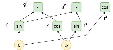
The sources of this graph represent the parameters of \(h\) (namely, \(\theta\) and \(\varphi\)). The sinks of this graph represent the top-most operations. Intermediate nodes represent intermediate operations. Thus, every non-sink node represents an operation. The graph is decomposed into "atomic" operations such as multiplication or trigonometric functions. The arrows in the graph indicate the inputs to operations.

The product of the respective Jacobian matrices is as follows:

\[\begin{bmatrix}\frac{\partial g^1}{\partial y^1}(f(\theta, \varphi)) & \frac{\partial g^1}{\partial y^2}(f(\theta, \varphi)) & \frac{\partial g^1}{\partial y^3}(f(\theta, \varphi)) & \frac{\partial g^1}{\partial y^4}(f(\theta, \varphi)) \\ \frac{\partial g^2}{\partial y^1}(f(\theta, \varphi)) & \frac{\partial g^2}{\partial y^2}(f(\theta, \varphi)) & \frac{\partial g^2}{\partial y^3}(f(\theta, \varphi)) & \frac{\partial g^2}{\partial y^4}(f(\theta, \varphi)) \\ \frac{\partial g^3}{\partial y^1}(f(\theta, \varphi)) & \frac{\partial g^3}{\partial y^2}(f(\theta, \varphi)) & \frac{\partial g^3}{\partial y^3}(f(\theta, \varphi)) & \frac{\partial g^3}{\partial y^4}(f(\theta, \varphi)) \end{bmatrix} \begin{bmatrix}\frac{\partial f^1}{\partial \theta}(\theta, \varphi) & \frac{\partial f^1}{\partial \varphi}(\theta, \varphi) \\ \frac{\partial f^2}{\partial \theta}(\theta, \varphi) & \frac{\partial f^2}{\partial \varphi}(\theta, \varphi) \\ \frac{\partial f^3}{\partial \theta}(\theta, \varphi) & \frac{\partial f^3}{\partial \varphi}(\theta, \varphi) \\ \frac{\partial f^4}{\partial \theta}(\theta, \varphi) & \frac{\partial f^4}{\partial \varphi}(\theta, \varphi)\end{bmatrix}\]

The resultant values are

\[\begin{bmatrix}\cos \varphi & \sin \theta & 0 & 0 \\ \sin \varphi & 0 & \sin \theta & 0 \\ 0 & 0 & 0 & 1\end{bmatrix}\begin{bmatrix}\cos \theta & 0 \\ 0 & -\sin \varphi \\ 0 & \cos \varphi \\ -\sin \theta & 0\end{bmatrix} = \begin{bmatrix}\cos \theta \cos \varphi & -\sin \theta \sin \varphi \\ \cos \theta \sin \varphi & \sin \theta \cos \varphi \\ -\sin \theta & 0\end{bmatrix}\]

Note that every term in the resultant product will be a sum of products of partial derivatives. For instance, the resultant term in row \(1\), column \(1\) will be

\[\frac{\partial g^1}{\partial y^1}(f(\theta, \varphi)) \cdot \frac{\partial f^1}{\partial \theta}(\theta, \varphi) + \frac{\partial g^1}{\partial y^2}(f(\theta, \varphi)) \cdot \frac{\partial f^2}{\partial \theta}(\theta, \varphi) + \frac{\partial g^1}{\partial y^3}(f(\theta, \varphi)) \cdot \frac{\partial f^3}{\partial \theta}(\theta, \varphi) + \frac{\partial g^1}{\partial y^4}(f(\theta, \varphi)) \cdot \frac{\partial f^4}{\partial \theta}(\theta, \varphi).\]

If we examine a single summand, such as

\[\frac{\partial g^1}{\partial y^1}(f(\theta, \varphi)) \cdot \frac{\partial f^1}{\partial \theta}(\theta, \varphi),\]

we notice that this product represents a distinct path within the graph. The "numerator" (component function) of each partial derivative indicates the sink and the "denominator" (coordinate function) of each partial derivative indicates the source of the operation represented by the respective component function. Products of partial derivatives indicate concatenations of paths. We will display paths in reverse order (i.e., starting at a sink and proceeding to a source). Thus, for instance, the previous term represents the following path (where intermediate nodes are labeled by their respective component functions and source nodes are labeled by parameters):

\[g^1 \rightarrow f^1 \rightarrow \theta.\]

Every summand in the terms in the resultant Jacobian matrix represents an alternative path. The sum itself represents every possible path from the respective source to the respective sink (e.g., in the example sum above, every path from from \(g^1\) to \(\theta\)).

Thus, we can systematically compute the derivatives using the chain rule by enumerating every possible path, computing the respective products representing each path, and accumulating the products in a sum at each respective source node.

1. \(g^1 \rightarrow \theta\). There is only one path: \(g^1 \rightarrow f^1 \rightarrow \theta\). This path is represented by \(\frac{\partial f^1}{\partial \theta}(\theta, \varphi) \cdot \frac{\partial g^1}{\partial y^1}(f(\theta, \varphi)) = \cos \theta \cos \varphi\).
2. \(g^1 \rightarrow \varphi\). There is only one path: \(g^1 \rightarrow f^2 \rightarrow \varphi\). This path is represented by \(\frac{\partial f^2}{\partial \varphi}(\theta, \varphi) \cdot \frac{\partial g^1}{\partial y^2}(f(\theta, \varphi)) = -\sin \theta \sin \varphi\).
3. \(g^2 \rightarrow \theta\). There is only one path: \(g^2 \rightarrow f^1 \rightarrow \theta\). This path is represented by \(\frac{\partial f^1}{\partial \theta}(\theta, \varphi) \cdot \frac{\partial g^2}{\partial y^1}(f(\theta, \varphi)) = \cos \theta \sin \varphi\).
4. \(g^2 \rightarrow \varphi\). There is only one path: \(g^2 \rightarrow f^3 \rightarrow \varphi\). This path is represented by \(\frac{\partial f^3}{\partial \varphi}(\theta, \varphi) \cdot \frac{\partial g^2}{\partial y^3}(f(\theta, \varphi)) = \sin \theta \cos \theta\).
5. \(g^3 \rightarrow \theta\). There is only one path: \(g^3 \rightarrow f^4 \rightarrow \theta\). Note that \(g^3\) was not depicted in the graph since it is the identity function, but and identity node could be added. This path is represented by \(\frac{\partial f^3}{\partial \theta}(\theta, \varphi) \cdot \frac{\partial g^3}{\partial y^4}(f(\theta, \varphi)) = -\sin \theta\).
6. \(g^3 \rightarrow \varphi\). There are no paths (so the result is \(0\)).

If we then write these in their respective position in the resultant matrix (where the entry \((i, j)\) at row \(i\) and column \(1\) is given by the product resulting from the path from \(g^i \rightarrow \theta\) and the entry at row \(i\) and column \(2\) is given by the product resulting form the path from \((g^i \rightarrow \varphi\)), we obtain the same result that we calculated previously from the product of Jacobian matrices.