The Darboux Integral

An integral is a continuous analog of a sum.

Finite Sums

Finite sums of real numbers can be defined in terms of a finite sequence \((a_i)_{i=0}^n\), i.e., a function \(a : I_n \rightarrow \mathbb{R}\) for a finite index set \(I_n = \{0,\dots,n\}\) where we write \(a_i\) for \(a(i)\).

We write the sum of such a finite sequence as

\[\sum_{i = 0}^n a_i.\]

Infinite Series

We can define the "sum" (i.e., series) of a countably infinite sequence of real numbers \((a_n)_{n \in \mathbb{N}}\) (i.e., a function \(a : \mathbb{N} \rightarrow \mathbb{R}\)) as the limit of the corresponding sequence \((s_k)_{k \in \mathbb{N}}\) of partial sums \(s_k = \sum_{i=0}^k a_i\), i.e.,

\[\sum_{i=0}^{\infty}a_i = \lim_{k \to \infty}s_k = \lim_{k \to \infty}\sum_{i=0}^k a_i.\]

Recall that such a limit, if it exists, is the unique real number \(L\) such that, for every real number \(\varepsilon \gt 0\) there exists a natural number \(N\) such that \(\lvert s_k - L\rvert \lt \varepsilon\) whenever \(k \ge N\).

Note that a series is not a true sum since there are infinitely many terms and the order of these terms might matter (for so-called conditionally convergent series), unlike finite sums. Instead, it represents the limit of a sequence of successively larger finite sums.

For instance, Euler's number \(e\) can be defined as the series

\[\sum_{i=0}^{\infty}\frac{1}{i!}.\]

As another example, in decimal notation, the number denoted as

\[0.\bar{9}\]

(i.e., with an infinite sequence of \(9\)'s) is exactly equal to \(1\), since the number denoted \(0.\bar{9}\) can be defined as the geometric series

\[\sum_{i=0}^{\infty}\frac{9}{10^{i+1}}\]

and

\[\lim_{k \to \infty}\sum_{i=0}^k \frac{9}{10^{i+1}} = 1,\]

i.e., the limit of the sequence

\[0.9, 0.99, 0.999,\dots\]

is \(1\).

Sums of Arbitrary Indexes

However, what does it mean to compute the "sum" of real numbers indexed by an arbitrary index set \(I\), i.e., the sum relative to a function \(a : I \rightarrow \mathbb{R}\), where \(a_i = a(i)\)? If the numbers are non-negative (i.e., \(a_i \ge 0\) for all \(i \in I\)) we can define the "sum" as the supremum of the sums of all finite subsets, i.e.,

\[\sum_{i \in I}a_i = \sup \left\{\sum_{i \in F}a_i : F \subseteq I, F ~\text{is finite}.\right\}\]

Thus, the "sum" is defined if and only if the corresponding supremum exists. However, it is possible to demonstrate that such a "sum" is defined only if all but at most countably many terms in the index are \(0\), i.e., the set

\[I^+ = \{i : a_i \gt 0\}\]

is either finite or countably infinite. To see this, note the following argument. Define a family of subsets of \(I^+_n\), one for each \(n \in \mathbb{N}\), as follows:

\[I^+_n = \left\{i \in I : a_i \gt \frac{1}{n}\right\}.\]

Every positive term \(a_i \gt 0\) must be a member of at least one such subset \(I^+_n\) since there exists an \(n \in \mathbb{N}\) such that \(a_i \gt 1/n\) for every term \(a_i\) (since such terms are positive). It thus follows that

\[I^+ = \bigcup_{n \in \mathbb{N}}I^+_n.\]

Suppose that \(I^+\) is uncountable. Then, since the countable union of finite sets is countable, if every set \(I^+_n\) were finite then \(I^+\) would be countable, which is a contradiction. Thus, at least one set \(I^+_n\) must be infinite. Since some \(I^+_n\) is infinite, we can select an arbitrary finite number of elements from it. Every element in \(I^+_n\) is at least \(1/n\). Let \(M\) be any positive real number. If we choose a finite subset \(F \subset I^+_n\) containing \(N\) elements where \(N \cdot (1/n) \gt M\), then

\[\sum_{i \in F}a_i \gt \sum_{i=1}^N \frac{1}{n} = N \cdot \frac{1}{n} \gt M.\]

Since \(M\) was arbitrary, the set

\[\left\{\sum_{i \in F}a_i : F \subseteq I, F ~\text{is finite}.\right\}\]

has no upper bound. This means that \(I^+\) cannot be uncountable, i.e., it must be countable.

Thus, we gain nothing with this particular notion of "sum", since it only applies to sets that are already countable anyway, and thus finite sums or infinite series are sufficient.

Integrals: The Idea

However, we would like some generalized analog of "sum" which applies to terms indexed by uncountable index sets. In particular, we will limit ourselves to index sets of the form \(I = [a, b]\) for some closed interval \([a,b]\) of real numbers. Thus, we want to define some analogous notion of "sum" for functions \(f : [a,b] \rightarrow \mathbb{R}\).

Although we cannot add the terms \(f(x)\) for \(x \in [a,b]\), we can add a weighted sum of a finite number of such terms, and then pass to a limit of such weighted sums.

In particular, we may think of the function \(f\) as a density. Recall that \(m = dv\) where \(m\) is mass, \(d\) is density, and \(v\) is volume, and, more generally, for multiple volumes \(v_i\) with respective densities \(d_i\),

\[m = \sum_i d_i \cdot v_i.\]

If we partition the interval \([a,b]\) into some number \(n\) of sub-intervals \([x_{i-1}, x_i]\) for \(i \in \{1,\dots,n\}\), we may think of the length \(x_i - x_{i-1}\) of each sub-interval as its "volume" (i.e., length is the one-dimensional analog of volume). We may then select some element \(t_i \in [x_{i-1},x_i]\) and think of \(f(t_i)\) as the "density" corresponding to the "volume" \(x_i - x_{i-1}\). We then arrive at the following weighted sum:

\[\sum_{i=1}^n f(t_i) \cdot (x_i - x_{i-1}).\]

The basic idea of the Darboux integral is as follows: first, partition the interval \([a,b]\) into a finite collection of (proper) sub-intervals \([x_{i-1}, x_i]\). A partition is a strictly-increasing finite sequence of \(n+1\) real numbers \((x_i)\) such that \(x_0 = a\) and \(x_n = b\), i.e., \(x_{i-1} < x_i\) for all \(i\) such that \(1 \le i \le n\). Then, define a "weighted sum"

\[\sum_{i=1}^n f(t_i) \cdot (x_i - x_{i-1})\]

where \(t_i\) is some representative element within the respective sub-interval (sometimes called a "tag"), i.e., \(t_i \in [x_{i-1}, x_i]\). Geometrically, each term in this sum represents the area of a rectangle with width \((x_i - x_{i-1})\) and height \(f(t_i)\). Geometrically, we may also view this weighted sum as an approximation of the area underneath the curve defined by \(f\) as bounded by the curve and the "x-axis" and limited to the interval \([a,b]\).

The Darboux integral defines two choices for \(t_i\): the upper value \(u_i\) is simply the supremum of the values of \(f\) over the respective sub-interval:

\[u_i = \sup\{f(x) : x \in [x_{i-1}, x_i] \}.\]

The lower value \(l_i\) is simply the infimum of the values of \(f\) over the respective sub-interval:

\[l_i = \inf\{f(x) : x \in [x_{i-1}, x_i] \}.\]

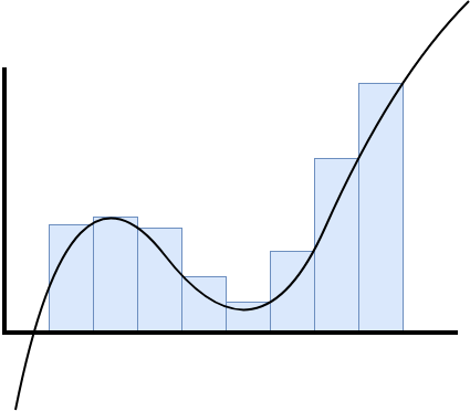
We can then define the upper sum as

\[U_{f,P} = \sum_{i=1}^n (x_i - x_{i-1}) \cdot u_i\]

and the lower sum as

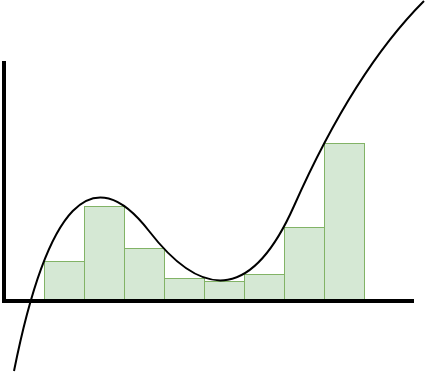
\[L_{f,P} = \sum_{i=1}^n (x_i - x_{i-1}) \cdot l_i,\]

where \(P = (x_i)\) is the sequence representing the endpoints of the sub-intervals within the respective partition and \(i \in \{0,\dots,n\}\) for some \(n \in \mathbb{N}\).

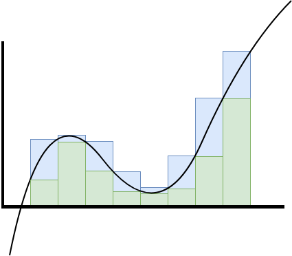
Thus, the lower sum is always less than or equal to the upper sum. The lower sum generally under-approximates the "true sum", and the upper sum generally over-approximates the "true sum".

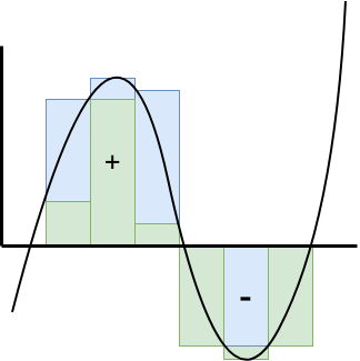
Also note that, for functions with negative values over the interval \([a,b]\), the sums "under the x-axis" will be negative, so we are dealing with a notion of signed area and densities that may be negative.

Given a partition \(P = (x_i)\) with \(n+1\) sub-intervals, we may refine this partition into a "finer" partition. A partition \(P' = (y_i)\) with \(m\) sub-intervals is a refinement of \(P\) if for every \(i\) with \(0 \le i \le n\), there exists an \(r(i) \in \mathbb{N}\) such that \(x_i = y_{r(i)}\).

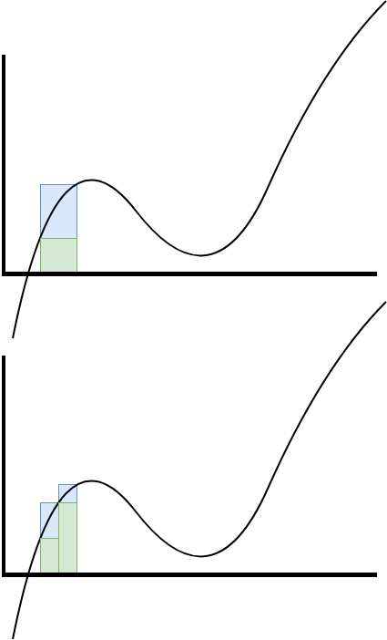
Each refinement reduces (or maintains) the upper sum and increases (or maintains) the lower sum. Thus, refinements generally reduce the error in the approximation. The idea is to refine the partitions indefinitely by considering all partitions and taking greatest lower bounds for upper sums and least upper bounds for lower sums.

When the greatest lower bound and least upper bound coincide, this represents the value we seek to compute, which we may think of as a weighted sum using \(f\) as a "density" and arbitrarily small volumes, or else as the area under the curve of \(f\).

The Definition

Thus, we define the upper Darboux integral as the infimum of all upper sums:

\[U_f = \inf\left\{U_{f,P} : P~\text{is a partition of}~[a,b]\right\}.\]

We likewise define the lower Darboux integral as the supremum of all lower sums:

\[L_f = \sup\left\{L_{f,P} : P~\text{is a partition of}~[a,b]\right\}.\]

We then finally define the Darboux integral as the unique real number denoted \(\int_a^b f\) such that the upper and lower Darboux integrals coincide, i.e.,

\[U_f = \int_a^b f = L_f.\]

If such a number exists, then the function \(f\) is said to be integrable on the respective interval \([a, b]\).

We summarize the definition formally as follows.

Definition (Darboux Integral). Let \(f : [a,b] \rightarrow \mathbb{R}\) be a function. A partition of the interval \([a,b]\) is a strictly increasing finite sequence of real numbers \((x_i)^n_{i = 0}\), such that \(x_0 = a\) and \(x_n = b\). The set of all partitions of an interval is denoted as \(\mathcal{P}([a,b])\). Given a partition \(P\), the respective lower Darboux sum is defined as

\[L_{f,P} = \sum_{i=1}^n (x_i - x_{i-1}) \cdot \inf\left\{f(x) : x \in [x_{i-1}, x_i]\right\}\]

and the respective upper Darboux sum is defined as

\[U_{f,P} = \sum_{i=1}^n (x_i - x_{i-1}) \cdot \sup\left\{f(x) : x \in [x_{i-1}, x_i]\right\}.\]

The lower Darboux integral is defined as

\[L_f = \sup\left\{L_{f,P} : P \in \mathcal{P}([a,b])\right\}\]

and the upper Darboux integral is defined as

\[U_f = \inf\left\{U_{f,P} : P \in \mathcal{P}([a,b])\right\}.\]

The Darboux integral of \(f\) on the interval \([a,b]\) is the unique real number denoted

\[\int_a^b f\]

such that

\[\int_a^b f = U_f = L_f.\]

If such a real number exists, then \(f\) is said to be integrable on the interval \([a,b]\).

Calculating Darboux Integrals

This definition precisely codifies one intuitive conception of integration. However, it is not immediately obvious how to compute concrete integrals. We thus consider a few properties of infima and suprema of sets of real numbers which will be useful for concrete calculations.

Theorem. The infimum \(p = \inf S\) of a set of real numbers \(S \subseteq \mathbb{R}\) exists if and only if \(p\) is a lower bound of \(S\) and for every \(\varepsilon \gt 0\) there exists an \(s \in S\) such that \(s \lt p + \varepsilon\).

Proof. Suppose that \(p = \inf S\) exists. Then, by definition, \(p\) is a lower bound of \(S\). Suppose that there exists some \(\varepsilon \gt 0\) such that \(s \ge p + \varepsilon\) for all \(s \in S\). Then \(p + \varepsilon\) is a lower bound of \(S\) and \(p \lt p + \varepsilon\) since \(\varepsilon \gt 0\), which contradicts the assumption that \(p\) is the greatest lower bound. Thus, for every \(\varepsilon \gt 0\), there exists an \(s \in S\) such that \(s \lt p + \varepsilon\).

Conversely, suppose that \(p\) is a lower bound of \(S\) and that for every \(\varepsilon \gt 0\) there exists an \(s \in S\) such that \(s \lt p + \varepsilon\). Suppose that there exists a lower bound \(p'\) of \(S\) such that \(p \lt p'\). Then, letting \(\varepsilon = p' - p\), since \(p \lt p'\) it follows that \(\varepsilon \gt 0\), and thus there exists an \(s \in S\) such that \(s \lt p + \varepsilon = p'\), which contradicts the assumption that \(p'\) is a lower bound. Therefore, there is no lower bound \(p'\) such that \(p \lt p'\), i.e., \(p\) is the greatest lower bound. \(\square\)

Theorem. The supremum \(p = \sup S\) of a set of real number \(S \subseteq \mathbb{R}\) exists if and only if \(p\) is an upper bound of \(S\) and for every \(\varepsilon \gt 0\) there exists an \(s \in S\) such that \(s \gt p - \varepsilon\).

Proof. Suppose that \(p = \sup S\) exists. Then, by definition, \(p\) is an upper bound of \(S\). Suppose that there exists some \(\varepsilon \gt 0\) such that \(s \le p - \varepsilon\) for all \(s \in S\). Then \(p - \varepsilon\) is an upper bound of \(S\) and \(p \gt p - \varepsilon\) since \(\varepsilon \gt 0\), which contradicts the assumption that \(p\) is the least upper bound. Thus, for every \(\varepsilon \gt 0\), there exists an \(s \in S\) such that \(s \gt p - \varepsilon\).

Conversely, suppose that \(p\) is an upper bound of \(S\) and that for every \(\varepsilon \gt 0\) there exists an \(s \in S\) such that \(s \gt p - \varepsilon\). Suppose that there exists an upper bound \(p'\) of \(S\) such that \(p \gt p'\). Then, letting \(\varepsilon = p - p'\), since \(p \gt p'\) it follows that \(\varepsilon \gt 0\), and thus there exists an \(s \in S\) such that \(s \gt p - \varepsilon = p'\), which contradicts the assumption that \(p'\) is an upper bound. Therefore, there is no upper bound \(p'\) such that \(p \gt p'\), i.e., \(p\) is the least upper bound. \(\square\)

Using these properties, we may establish the following useful characterization of Darboux integrable functions.

Theorem. A function \(f : [a, b] \rightarrow \mathbb{R}\) is Darboux integrable if and only if for every \(\varepsilon \gt 0\) there exists a partition \(P\) of \([a, b]\) such that

\[U_{f,P} - L_{f,P} \lt \varepsilon.\]

Proof. Suppose that for every \(\varepsilon \gt 0\) there exists a partition \(P\) of \([a,b]\) such that \(U_{f,P} - L_{f,P} \lt \varepsilon\). Since \(U_f \le U_{f,P}\) and \(L_f \ge L_{f,P}\) and \(U_f \ge L_f\), it follows that \(0 \le U_f - L_f \lt \varepsilon\). If \(U_f - L_f \gt 0\), then, choosing \(\varepsilon = U_f - L_f\), it follows that \(U_f - L_f \lt \varepsilon = U_f - L_f\), a contradiction. Thus, \(U_f - L_f = 0\), i.e., \(U_f = L_f\), and hence \(f\) is Darboux integrable.

Conversely, suppose that \(f\) is Darboux integrable. Then \(p = U_f = L_f\). Suppose \(\varepsilon \gt 0\). Then there exists a partition \(P_1\) of \([a,b]\) such that \(U_{f,P_1} \lt p + \frac{\varepsilon}{2}\) and there exists a partition \(P_2\) of \([a,b]\) such that \(L_{f,P_2} \gt p - \frac{\varepsilon}{2}\). There exists a common refinement \(P\) of \(P_1\) and \(P_2\) and thus since \(U_{f,P} \le U_{f,P_1}\) and \(L_{f,P} \ge L_{f,P_1}\) it follows that \(U_{f,P} \lt p + \frac{\varepsilon}{2}\) and \(L_{f,P} \gt p - \frac{\varepsilon}{2}\). Since \(U_{f,P} \gt L_{f,P}\) and each exist within the interval \((p - \frac{\varepsilon}{2}, p + \frac{\varepsilon}{2})\), it thus follows that

\[U_{f,P} - L_{f,P} \lt 2 \cdot \frac{\varepsilon}{2} = \varepsilon.\]

\(\square\)

Example

First, we will consider the example of a function \(f : [a, b] \rightarrow \mathbb{R}\) which is non-zero (i.e. equals \(y\) for some \(y \gt 0\)) only at a single point \(x^+\) in its domain:

\[f(x) = \begin{cases}y, & x = x^+ \\ 0 & x \ne x^+.\end{cases}\]

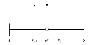
We will assume that \(x^+ \in [a,b]\); otherwise, the value of the integral will be \(0\) immediately since \(f(x) = 0\) everywhere except at \(x^+\). We will also assume that \(x^+ \gt 0\). Note that, no matter which partition \(P\) we work with, there must be some interval \([x_{j-1}, x_j]\) for some index \(0 \le j \le n\) containing \(x^+\), and on this interval \(l_j = 0\) and \(u_j = y\). On all other intervals where \(i \ne j\), \(l_i = u_i = 0\). It thus follows that

\[L_{f,P} = \sum_{i=1}^n l_i \cdot (x_i - x_{i-1}) = 0\]

and

\begin{align*}U_{f,P} &= \sum_{i=1}^n u_i \cdot (x_i - x_{i-1}) \\&= \sum_{i=1}^{j-1} u_i \cdot (x_i - x_{i-1}) \\&+ u_i \cdot (x_j - x_{j-1}) \\&+ \sum_{i=j+1}^n u_i \cdot (x_i - x_{i-1}) \\&= 0 + y \cdot (x_j - x_{j-1}) + 0 \\&= y \cdot (x_j - x_{j-1}).\end{align*}

Thus, \(U_{f,P} - L_{f,P} = x_j - x_{j-1}\). Therefore, for any \(\varepsilon \gt 0\), if we select a partition \(P\) with \(x_{j-1} \lt x^+ \lt x_j\) and \(y \cdot (x_j - x_{j-1}) \lt \varepsilon\), then

\[U_{f,P} - L_{f,P} \lt \varepsilon,\]

and hence \(f\) is integrable. Since \(L_{f,P} = 0\) for any partition \(P\) whatsoever, it follows that \(L_f = 0\) and hence

\[\int_a^b f = 0.\]

Thus, the integral of any function that is non-zero at a single point in its domain is \(0\). This matches our intuition: geometrically, the figure represented by the graph has zero area.

Example

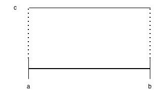
Next, let's consider the example of a constant function \(f: [a,b] \rightarrow \mathbb{R}\) such that, for some \(c \in \mathbb{R}\), \(f(x) = c\) for all \(x \in [a,b]\).

We expect the integral to be equal to \(c \cdot (b - a)\) since the graph of \(f\) is a rectangle with width \(b-a\) and height \(c\) which has area \(c \cdot (b-a)\).

For any partition \(P\) whatsoever, \(u_i = l_i = c\) for all \(i\). Thus,

\begin{align*}L_{f,P} &= U_{f,P} \\&= \sum_{i=1}^n c \cdot (x_i - x_{i-1}) \\&= c \cdot \sum_{i=1}^n (x_i - x_{i-1}) \\&= c \cdot (b-a).\end{align*}

Then, for any \(\varepsilon \gt 0\), \(U_{f,P} - L_{f,P} = 0 \lt \varepsilon\), so \(f\) is integrable. Furthermore, \(U_f = L_f = c \cdot (b-a)\), and so

\[\int_a^bf = c \cdot (b-a).\]

Example

Next, let's consider the example of the function \(f : [a,b] \rightarrow \mathbb{R}\) with \(f(x) = x\) for all \(x \in [a,b]\). For the sake of simplicity, we will assume that \(a \gt 0\).

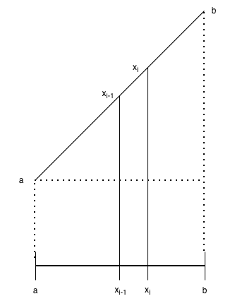
We expect the integral to be the sum of the area of the right triangle and rectangle as depicted in the figure, namely

\[\frac{1}{2} \cdot (b-a)^2 + (b-a) \cdot a = \frac{b^2}{2} - \frac{a^2}{2}.\]

Note that on any interval \([x_{i-1},x_i]\), \(l_i = x_{i-1}\) and \(u_i = x_i\). If we choose a partition \(P\) which partitions \([a,b]\) into \(n\) intervals of equal length \(\frac{b-a}{n}\), then \(x_0 = a\), \(x_1 = a + \frac{b-a}{n}\), \(x_2 = a + 2 \cdot \frac{b-a}{n}\), etc., and in general \(x_i = a + i \cdot \frac{b-a}{n}\).

Observe that

\begin{align*}L_{f,P} &= \sum_{i=1}^n l_i \cdot (x_i - x_{i-1}) \\&= \sum_{i=1}^n x_{i-1} \cdot (x_i - x_{i-1}) \\&= \sum_{i=1}^n \left(a + (i-1) \cdot \frac{b-a}{n}\right) \cdot \frac{b-a}{n} \\&= \sum_{i=1}^n \left(a \cdot \frac{b-a}{n} + (i-1) \cdot \frac{(b-a)^2}{n^2}\right) \\&= \left(\sum_{i=1}^n a \cdot \frac{b-a}{n}\right) + \left(\sum_{i=1}^n (i-1) \cdot \frac{(b-a)^2}{n^2}\right) \\&= a \cdot (b-a) + \frac{(b-a)^2}{n^2} \cdot \sum_{i=1}^n (i-1) \\&= a \cdot (b-a) + \frac{(b-a)^2}{n^2} \cdot \sum_{j=0}^{n-1}j \\&= a \cdot (b-a) + \frac{(b-a)^2}{n^2} \cdot \frac{n(n-1)}{2} \\&= a \cdot (b-a) + \frac{(b-a)^2}{2} \cdot \frac{n-1}{n} \\&= \frac{n}{n-1} \cdot \frac{n-1}{n} \cdot a \cdot (b-a) + \frac{(b-a)^2}{2} \cdot \frac{n-1}{n} \\&= \frac{n-1}{n} \cdot \left(\frac{n}{n-1}a \cdot (b-a) + \frac{(b-a)^2}{2}\right) \\&= \frac{n-1}{n} \cdot \left(\frac{1}{n-1}a \cdot (b-a) + a \cdot (b-a) + \frac{(b-a)^2}{2}\right) \\&= \frac{n-1}{n} \cdot \left(\frac{1}{n-1}a \cdot (b-a) + \frac{b^2 - a^2}{2}\right) \\&= \frac{a(b-a)}{n} + \frac{n-1}{n} \cdot \frac{b^2 - a^2}{2}. \end{align*}

A similar calculation shows that

\[U_{f,P} = \frac{a(b-a)}{n} + \frac{n+1}{n} \cdot \frac{b^2 - a^2}{2}.\]

It follows that

\[U_{f,P} - L_{f,P} = \frac{b^2 - a^2}{n}.\]

For any \(\varepsilon \gt 0\), we can choose a value of \(n\) such that

\[\frac{b^2 - a^2}{n} \lt \varepsilon,\]

so \(f\) is integrable.

Next, note that, since \(b \gt a\) it follows that \(0 \lt (b-a)^2\) and thus

\[0 \lt a^2 - 2ab + b^2.\]

From this, we can infer that

\[a(b-a) \lt \frac{b^2 - a^2}{2}.\]

It then follows that

\begin{align*}L_{f,P} &= \frac{a(b-a)}{n} + \frac{n-1}{n} \cdot \frac{b^2 - a^2}{2} \\&\lt \frac{b^2 - a^2}{2n} + \frac{n-1}{n} \cdot \frac{b^2 - a^2}{2} \\&= \frac{b^2 - a^2}{2}.\end{align*}

It is clear that

\[U_{f,P} \gt \frac{b^2 - a^2}{2},\]

and thus

\[L_{f,P} \lt \frac{b^2 - a^2}{2} \lt U_{f,P}.\]

Since \(U_{f,P} - L_{f,P}\) can be made arbitrarily small by choosing a sufficiently large number of partitions \(n\), it follows that there is only one number between \(L_{f,P}\) and \(U_{f,P}\) and thus \(U_f = L_f = (b^2 - a^2) / 2\). To see this, consider the following argument. If \(L_f \lt (b^2 - a^2)/2\), then \(\varepsilon = (b^2 - a^2)/2 - L_f \gt 0\), and thus there exists a partition \(P\) such that \(U_{f,P} - L_{f,P} \lt \varepsilon = (b^2 - a^2)/2 - L_f\), which, since \(L_{f,P} \lt L_f\), then implies that \(U_{f,P} - L_f \lt (b^2 - a^2)/2 - L_f\) and hence \(U_{f,P} \lt (b^2 - a^2)/2\), which is a contradiction. Thus, \(L_f \ge (b^2 - a^2)/2\). A similar argument shows that \(U_f \ge (b^2 - a^2)/2\). Thus

\[L_f \le (b^2 - a^2)/2 \le U_f,\]

and since \(U_f = L_f\), this implies that \(U_f = L_f = (b^2 - a^2)/2\).

Thus, we have shown that

\[\int_a^b f = \frac{b^2}{2} - \frac{a^2}{2}.\]

Example

Thus far, the examples have been fairly trivial: they computed values which could have been computed much more easily by more elementary techniques. However, they serve as useful confirmations that the integral works as intended. Now we will consider a non-trivial example: the function \(f(x) = x^2\).

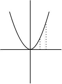
We will assume, for the sake of simplicity, that \(a = 0\), i.e., we are working on the interval \([0, b]\). On any partition of \([0,b]\), \(l_i = x_{i-1}^2\) and \(u_i = x_i^2\). Once again, we choose a partition \(P\) of \([0,b]\) consisting of \(n\) sub-intervals of equal length, so that

\[x_i = i \cdot \frac{b}{n}.\]

We compute \(L_{f,P}\) as follows:

\begin{align*}L_{f,P} &= \sum_{i=1}^n x_{i-1}^2 \cdot (x_i - x_{i-1}) \\&= \sum_{i=1}^n \left((i-1) \cdot \frac{b}{n}\right)^2 \cdot \frac{b}{n} \\&= \sum_{i=1}^n (i-1)^2 \cdot \frac{b^3}{n^3} \\&= \frac{b^3}{n^3} \cdot \sum_{i=1}^n (i-1)^2 \\&= \frac{b^3}{n^3} \cdot \sum_{j=0}^{n-1} j^2 \\&= \frac{b^3}{n^3} \cdot \frac{1}{6} \cdot (n-1)(n)(2n-1).\end{align*}

The ultimate equation uses the fact that

\[\sum_{j=0}^k k^2 = \frac{1}{6}(k)(k+1)(2k+1).\]

We compute \(U_{f,P}\) as follows:

\begin{align*}U_{f,P} &= \sum_{i=1}^n x_i^2 \cdot (x_i - x_{i-1}) \\&= \sum_{i=1}^n \left(i \cdot \frac{b}{n}\right) \cdot \frac{b}{n} \\&= \sum_{i=1}^n i^2 \cdot \frac{b^3}{n^3} \\&= \frac{b^3}{n^3} \cdot \sum_{i=1}^n i^2 \\&= \frac{b^3}{n^3} \cdot \frac{1}{6} \cdot (n)(n+1)(2n+1).\end{align*}

Continuing, we compute

\[L_{f,P} = \frac{b^3}{3} - \frac{b^3}{2n} + \frac{b^3}{6n^2}.\]

The terms containing \(n\) in the denominator vanish as \(n\) becomes arbitrarily large, so the only non-vanishing term is

\[\frac{b^3}{3}.\]

Since, for all \(n\),

\[\frac{b^3}{6n^2} \lt \frac{b^3}{2n},\]

it follows that

\[- \frac{b^3}{2n} + \frac{b^3}{6n^2} \lt 0\]

and thus

\[L_{f,P} \lt \frac{b^3}{3}.\]

A similar calculation shows that

\[U_{f,P} = \frac{b^3}{3} + \frac{b^3}{2n} + \frac{b^3}{6n^2}.\]

The terms containing \(n\) in the denominator vanish as \(n\) becomes arbitrarily large, so the only non-vanishing term is again

\[\frac{b^3}{3}.\]

Clearly,

\[U_{f,P} \gt \frac{b^3}{3}.\]

Thus,

\[L_{f,P} \lt \frac{b^3}{3} \lt U_{f,P}.\]

Then,

\[U_{f,P} - L_{f,P} = \frac{b^3}{n},\]

which can be made arbitrarily small. Thus, \(f\) is integrable. A similar argument to the argument employed in previous examples then shows that

\[\int_0^b f = \frac{b^3}{3}.\]

Conclusion

The example calculations indicate that it can be fairly difficult to compute integrals directly. Instead, one typically proceeds by proving various general theorems and then applying these theorems to compute integrals. One of the most important such theorems is the fundamental theorem of calculus which relates derivatives to integrals, indicating that, in a certain sense, they are inverses of one another. This provides a means of computing many integrals.