The Euclidean Metric in Spherical Coordinates

This post discusses the derivation of the expression for the Euclidean metric in spherical coordinates.

Spherical Coordinates on Euclidean Space

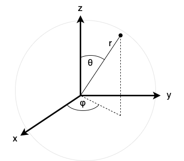
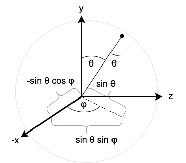
First, it is instructive to review spherical coordinates. Spherical coordinates \((r,\theta,\varphi)\) identify points in \(\mathbb{R}^3\) as a combination of a radial distance \(r\) from the origin, a polar angle \(\theta\) which indicates the declination from the polar axis, and an azimuthal angle which indicates the rotation about the polar axis, as in Figure 1.

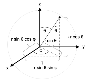
The following mapping maps spherical coordinates to Cartesian (x, y, z) coordinates, as depicted in Figure 2:

\[(r,\theta,\varphi) \mapsto (r \sin \theta \cos \varphi, r \sin \theta \sin \varphi, r \cos \theta).\]

However, for these coordinates to be unique, they must be restricted such that \(r \in (0,\infty)\), \(\theta \in (0,\pi)\), and \(\varphi \in (0,2\pi)\). Additionally, we require that each domain be an open interval of \(\mathbb{R}\).

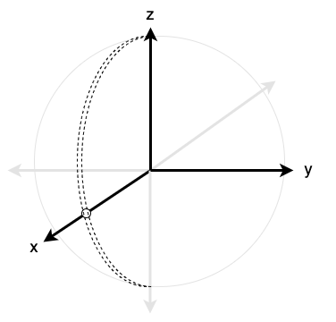
This means that there is a "gap" in each sphere since some coordinates are excluded (wherever \(r=0\), \(\theta = 0\), \(\theta = \pi\) \(\varphi = 0\), \(\varphi = 2\pi\), etc.), as in Figure 3.

Thus, when considering all spheres of all radii \(r \gt 0\) and considering the fact that \(r=0\) is excluded, the following half plane is missing from the codomain of the mapping of spherical coordinates to Cartesian coordinates:

\[H_{x,z} = \{(x,y,z) \in \mathbb{R}^3 : x \ge 0, y = 0\}.\]

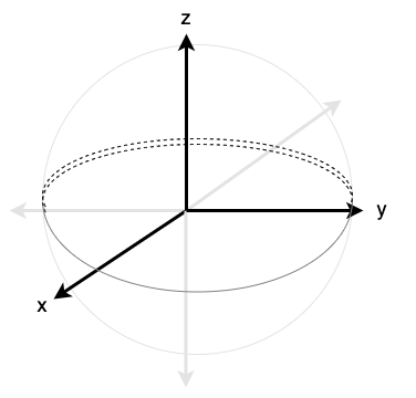
To compensate, perpendicular spherical coordinates can be used which contain a "gap" which is "perpendicular" to the "gap" from standard spherical coordinates, as in Figure 4.

The perpendicular spherical coordinates designate a different polar axis and have corresponding angular conventions, as in Figure 5.

Thus, the mapping of perpendicular spherical coordinates to Cartesian coordinates is defined as follows:

\[(r,\theta,\varphi) \mapsto (-r\sin \theta \cos \varphi, r\cos \theta, r\sin \theta \sin \varphi).\]

Thus, when considering all spheres of all radii \(r \gt 0\) and considering the fact that \(r=0\) is excluded, the following half plane is missing from the codomain of the mapping of perpendicular spherical coordinates to Cartesian coordinates:

\[H_{-x,y} = \{(x,y,z) \in \mathbb{R}^3 : x \le 0, z = 0\}.\]

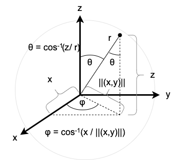
These mappings are bijective, and thus they have inverses. The inverse mapping from Cartesian coordinates to spherical coordinates is defined as follows (and is depicted in Figure 6):

\[(x,y,z) \mapsto \begin{cases}\left(\sqrt{x^2 + y^2 + z^2}, \cos^{-1}\left(\frac{z}{\sqrt{x^2 + y^2 + z^2}}\right),\cos^{-1}\left(\frac{x}{\sqrt{x^2 + y^2}}\right) \right) & \text{if}~y \gt 0~\text{or if}~y=0~\text{and}~x \lt 0, \\ \left(\sqrt{x^2 + y^2 + z^2}, \cos^{-1}\left(\frac{z}{\sqrt{x^2 + y^2 + z^2}}\right), \pi + \cos^{-1}\left(\frac{-x}{\sqrt{x^2 + y^2}}\right) \right) & \text{if}~y \lt 0.\end{cases}\]

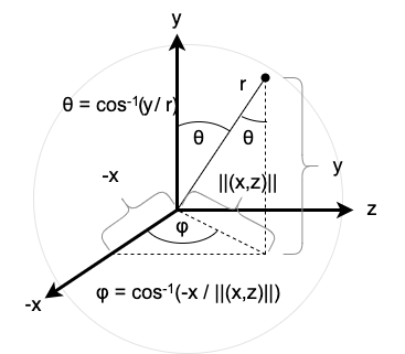
Likewise, the inverse mapping from Cartesian coordinates to perpendicular spherical coordinates is defined as follows (and is depicted in Figure 7):

\[(x,y,z) \mapsto \begin{cases}\left(\sqrt{x^2 + y^2 + z^2}, \cos^{-1}\left(\frac{y}{\sqrt{x^2 + y^2 + z^2}}\right),\cos^{-1}\left(\frac{-x}{\sqrt{x^2 + z^2}}\right) \right) & \text{if}~z \gt 0~\text{or if}~z=0~\text{and}~x \gt 0, \\ \left(\sqrt{x^2 + y^2 + z^2}, \cos^{-1}\left(\frac{y}{\sqrt{x^2 + y^2 + z^2}}\right), \pi + \cos^{-1}\left(\frac{x}{\sqrt{x^2 + z^2}}\right) \right) & \text{if}~z \lt 0.\end{cases}\]

Thus, if we denote the mapping from Cartesian coordinates to spherical coordinates as \(\varphi\) (and the mapping from spherical coordinates to Cartesian coordinates as \(\varphi^{-1}\)) and the mapping from Cartesian coordinates to perpendicular spherical coordinates as \(\psi\) (and the mapping from perpendicular spherical coordinates to Cartesian coordinates as \(\psi^{-1}\)), then we can construct an atlas for \(\mathbb{R}^3 \setminus \{0\}\) consisting of the following charts:

• \((\mathbb{R}^3 \setminus H_{x,z}, \varphi)\),
• \((\mathbb{R}^3 \setminus H_{-x,y}, \psi)\).

This is indeed an atlas since \(\mathbb{R}^3 \setminus \{0\} = (\mathbb{R}^{3} \setminus H_{x,z}) \cup (\mathbb{R}^3 \setminus H_{-x,y})\), and \(\varphi\) and \(\psi\) are bijections onto their common image \((0,\infty) \times (0,\pi) \times (0,2\pi)\) which is an open set in \(\mathbb{R}^3\). The transition maps \(\varphi \circ \psi^{-1}\) and \(\psi \circ \varphi^{-1}\) coincide, and are smooth functions defined as follows:

\[(\theta, \varphi) \mapsto \begin{cases}\left(\cos^{-1}(\sin \theta \sin \varphi), \cos^{-1}\left(\frac{-\sin \theta \cos \varphi}{\sqrt{\sin^2 \theta \cos^2 \varphi + \cos^2 \theta}}\right)\right) & \text{if}~\cos \theta \gt 0 ~\text{or if}~ \cos \theta = 0 ~\text{and}~ \cos \varphi \gt 0 \\ \left(\cos^{-1}(\sin \theta \sin \varphi), \pi + \cos^{-1}\left(\frac{\sin \theta \cos \varphi}{\sqrt{\sin^2 \theta \cos^2 \varphi + \cos^2 \theta}}\right)\right)& \text{if}~ \cos \theta \lt 0.\end{cases}\]

The "spheres" described above don't really have the desired "shape" unless the manifold is endowed with the Euclidean metric, which, in standard coordinates (in the admissible chart \((\mathbb{R} \setminus \{0\}, \mathrm{id})\) where the component functions of \(\mathrm{id}\) are written as \(x\), \(y\), and \(z\)) takes the form

\[g = dx^2 + dy^2 + dz^2\]

so that, at each point \(p \in \mathbb{R} \setminus \{0\}\) and for each tangent vector \(v\) at \(p\), the norm of each tangent vector is given by its Euclidean norm:

\[\lVert v \rVert = \sqrt{g_p(v,v)} = \sqrt{dx_p^2(v) + dy_p^2(v) + dz_p^2(v)} = \sqrt{(v^x)^2 + (v^y)^2 + (v^z)^2}.\]

It is useful to express this metric in spherical coordinates. One method of doing so involves the pullback of the metric \(g\). If we treat the chart domain \(\mathbb{R}^3 \setminus H_{x,y}\) as a manifold equipped with the Euclidean metric, we can pull back the metric \(g\) along the map \(\varphi^{-1}\) resulting in the pullback \((\varphi^{-1})^*g\). Since \(\varphi^{-1}\) is a diffeomorphism (all chart maps are diffeomorphisms onto their images), the pullback \((\varphi^{-1})^*g\) itself is a metric on the manifold \((0,\infty) \times (0,\pi) \times (0,2\pi)\). If we define the pullback metric \((\varphi^{-1})^*g\) as the metric on this manifold, then \(\varphi^{-1}\) becomes an isometry by definition (recall that two manifolds are isometric if there exists a diffeomorphism between them such that the pullback of one's metric along this diffeomorphism is equal to the other's metric). We can then pull back along \(\varphi\), which, by the properties of pullbacks, yields

\[\varphi^*((\varphi^{-1})^*g) = (\varphi^{-1} \circ \varphi)^*g = \mathrm{id}^*g = g.\]

This might not seem to achieve anything since it yields the original metric \(g\), yet, if we compute the coordinate expressions for each of these pullbacks, it will yield a coordinate expression for \(g\) in spherical coordinates.

Recall that, if \(F : M \rightarrow N\) is a smooth map between smooth manifolds \(M\), \(N\) and \(B\) is a covariant tensor field on \(N\), \((y^i)\) are smooth coordinates defined on a neighborhood \(U\) of \(F(p)\) for a point \(p \in M\), then \(F^*B\) has the following coordinate expression:

\begin{align}F^*B &= F^*(B_{i_1,\dots,i_k}dy^{i_1} \otimes \dots \otimes dy^{i_k}) \\&= (B_{i_1,\dots,i_k} \circ F)d(y^{i_1} \circ F) \otimes \dots \otimes d(y^{i_k} \circ F)\end{align}

In other words, pullbacks operate by substitution (since composition can model substitution): simply substitute the \(i\)-th component function of \(F\) in these coordinates for \(y^i\) and \(B_{i_1,\dots,i_k}\) everywhere.

In particular, the pullback of an arbitrary metric \(g\) has the form

\begin{align}F^*g &= F^*(g_{ij}dy^{i} \otimes dy^{j}) \\&= (g_{ij}\circ F)d(y^{i} \circ F) \otimes d(y^{j} \circ F).\end{align}

Thus, in the example of the Euclidean metric, which may be written as

\[g_{xx} dx \otimes dx + g_{yy} dy \otimes dy + g_{zz} dz \otimes dz\]

where each of the functions \(g_{xx}\), \(g_{yy}\), and \(g_{zz}\) are all the constant function \(1\), it follows that the pullback metric \((\varphi^{-1})^*g\) may be calculated in terms of standard coordinates as follows:

\begin{align}(\varphi^{-1})^*g &= (\varphi^{-1})^*(g_{xx} dx \otimes dx + g_{yy} dy \otimes dy + g_{zz} dz \otimes dz) \\&= (\varphi^{-1})^*(1 dx^2 + 1 dy^2 + 1 dz^2) \\&= (1 \circ \varphi^{-1})d(x \circ \varphi^{-1})^2 + (1\circ \varphi^{-1})d(y \circ \varphi^{-1})^2 + (1 \circ \varphi^{-1})d(z \circ \varphi^{-1})^2 \\&= d(r \sin \theta \cos \varphi)^2 + d(r \sin \theta \sin \varphi)^2 + d(r\cos \theta)^2 \\&= (\sin\theta\cos\varphi dr + r\cos\theta\cos\varphi d\theta - r\sin\theta\sin\varphi d\varphi)^2 \\&+ (\sin\theta\sin\varphi dr + r\cos\theta\sin\varphi d\theta + r\sin\theta\cos\varphi d\varphi)^2 \\&+ (\cos\theta dr - r\sin\theta d\theta)^2 \\&= (\sin^2\theta\cos^2\varphi dr^2 \\&+ 2r\cos\theta\sin\theta\cos^2\varphi dr d\theta \\&- 2r \sin^2\theta\cos\varphi\sin\varphi dr d\varphi \\&+ r^2 \cos^2\theta\cos^2\varphi d\theta^2 \\&- 2r^2\cos\theta\sin\theta\cos\varphi\sin\varphi d\theta d\varphi \\&+ r^2\sin^2\theta\sin^2\varphi d\varphi^2) \\&+ (\sin^2\theta\sin^2\varphi dr^2 \\&+ 2r\sin\theta\cos\theta\sin^2\varphi dr d\theta \\&+ 2r\sin^2\theta\cos\varphi\sin\varphi dr d\varphi \\&+ r^2\cos^2\theta\sin^2\varphi d\theta^2 \\&+ 2r^2\cos\theta\sin\theta\cos\varphi\sin\varphi d\theta d\varphi \\&+ r^2\sin^2\theta\cos^2\varphi d\varphi^2) \\&+ (\cos^2\theta dr^2 \\&- 2r\cos\theta\sin\theta dr d\theta \\&+ r^2\sin^2\theta d\theta^2) \\&= (\sin^2\theta\cos^2\varphi + \sin^2\theta\sin^2\varphi d\theta^2 + \cos^2\theta)dr^2 \\&+ (2r\cos\theta\sin\theta\cos^2\varphi + 2r\cos\theta\sin\theta\sin^2\varphi - 2r\cos\theta\sin\theta)dr d\theta \\&+ (r^2\cos^2\theta\cos^2\varphi + r^2\cos^2\theta\sin^2\varphi + r^2\sin^2\theta)d\theta^2 \\&+ (r^2\sin^2\theta\sin^2\varphi + r^2\sin^2\theta\cos^2\varphi)d\varphi^2 \\&= (\sin^2\theta(\cos^2\varphi + \sin^2\varphi) + \cos^2\theta)dr^2 \\&+ (2r\cos\theta\sin\theta(\cos^2\varphi + \sin^2\varphi) - 2r\cos\theta\sin\theta)dr d\theta \\&+ (r^2\cos^2\theta(\cos^2\varphi + \sin^2\varphi) + r^2\sin^2\theta)d\theta^2 \\&+ (r^2\sin^2\theta(\sin^2\varphi + \cos^2\varphi))d\varphi^2 \\&= (\sin^2\theta + \cos^2\theta)dr^2 \\&+ (2r\cos\theta\sin\theta - 2r\cos\theta\sin\theta)dr d\theta \\&+ (r^2\cos^2\theta + r^2\sin^2\theta)d\theta^2 \\&+ (r^2\sin^2\theta)d\varphi^2 \\&= dr^2 \\&+ (r^2(\cos^2\theta + \sin^2\theta))d\theta^2 \\&+ (r^2\sin^2\theta)d\varphi^2 \\&= dr^2 + r^2 d\theta^2 + (r^2\sin^2\theta)d\varphi^2.\end{align}

The metric \((\varphi^{-1})^*g\) is a metric on \((0,\infty) \times (0,\pi) \times (0, 2\pi)\). Since we desire a metric on \(\mathbb{R}^3 \setminus \{0\}\), we need to pull back again along \(\varphi\). Writing \(\varphi\) in terms of the coordinates \((r,\theta,\varphi)\) as

\[\varphi(x,y,z) = (r(x,y,z),\theta(x,y,z),\varphi(x,y,z)),\]

the pullback metric \(\varphi^*((\varphi^{-1})^*g) = g\) in these coordinates may also be written as

\[g = dr^2 + r^2 d\theta^2 + (r^2\sin^2\theta)d\varphi^2,\]

noting that \(r\), \(\theta\), and \(\varphi\) now denote the coordinate functions on \(\mathbb{R}^3 \setminus \{0\}\) defined as

• \(r(x,y,z) = \sqrt{x^2 + y^2 + z^2}\),
• \(\theta(x,y,z) = \cos^{-1}z\),
• \(\varphi(x,y,z) = \begin{cases}\cos^{-1}\left(\frac{x}{\sqrt{x^2 + y^2}}\right) & \text{if} \\ \pi + \cos^{-1}\left(\frac{-x}{\sqrt{x^2 + y^2}}\right) & \text{if}\end{cases}\)

whereas in the coordinate expression for the metric \((\varphi^{-1})^*g\), the coordinate functions \(r\), \(\theta\), and \(\varphi\) on \((0,\infty) \times (0,\pi) \times (0,2\pi)\) were simply the component functions of \(\mathrm{id}\), namely

• \(r(r,\theta,\varphi) = r\),
• \(\theta(r,\theta,\varphi) = \theta\),
• \(\varphi(r,\theta,\varphi) = \varphi\)

and we have implicitly substituted one for the other in the pullback.

Note that in perpendicular spherical coordinates, the metric assumes the same coordinate expression, but the functions \(r\), \(\theta\), and \(\varphi\) have different definitions since they refer to different coordinates.