The Real Numbers

What are the real numbers? What are numbers for that matter? This might seem like a philosophical question rather than a mathematical question, but, as Gottlob Frege famously quipped

“Every good mathematician is at least half a philosopher, and every good philosopher is at least half a mathematician.”
― Gottlob Frege

Such questions are inescapable if we are to examine mathematics rigorously. For instance, what is the length of the hypotenuse of the following right triangle?

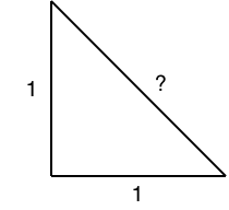
Of course, the Pythagorean theorem indicates that it is \(\sqrt{2}\). But what sort of number is \(\sqrt{2}\)? Consider the following famous theorem.

Theorem. \(\sqrt{2}\) is irrational.

Proof. Suppose that \(\sqrt{2}\) is rational. Then, by definition, there exist non-zero integers \(p\) and \(q\) such that

\[\sqrt{2} = \frac{p}{q}.\]

We may assume that \(p\) and \(q\) have no common divisors (i.e., the ratio \(\frac{p}{q}\) is reduced). It follows that \(2 = \frac{p^2}{q^2}\) and thus \(2q^2 = p^2\). Thus, by definition, \(p^2\) is even and so is \(p\) and so, by definition, there exists an integer \(k\) such that \(p = 2k\). Then,

\begin{align*}2q^2 &= p^2 \\&= (2k)^2 \\&= 4k^2\end{align*}

and thus \(q^2 = 2k^2\) and \(q\) is even. Since both \(p\) and \(q\) are even, they have a common divisor (namely, \(2\)). This contradicts the assumption that \(p\) and \(q\) have no common divisor. Thus, no such integers \(p\) and \(q\) exist, i.e., \(\sqrt{2}\) is not rational. \(\square\)

Thus, even if we take for granted the notions of integer and rational number and multiplication and square root, we still must explain what we mean by an irrational number. We have said what irrational numbers aren't, but we haven't said what they are.

In fact, the real numbers are precisely what we obtain when we combine the set of rational numbers with the set of irrational numbers.

Intuitively, the real numbers represent continuous quantities, i.e., there is an infinitude of intermediate real numbers between any two real numbers. However, this is also true of the rational numbers: for instance, between any rational numbers \(p\) and \(q\) with \(p \lt q\) there is the midpoint \(m_1 = p + \frac{q-p}{2}\), and between \(p\) and \(m_1\) there is another midpoint \(m_2 = p + \frac{m_1-p}{2}\), and this process of subdivision can continue indefinitely. However, we will later discover that this intervening infinitude of real numbers is uncountable whereas the intervening infinitude of rational numbers is countable; this is one sense in which the real numbers are "continuous".

Intuitively, there are no "gaps" or "holes" in the real numbers (where \(\sqrt{2}\) is an example of a number "missing" from the rational numbers). In other words, the real numbers are complete. But complete with respect to what? Consider the following theorem.

Theorem. The set

\[S = \{q \in \mathbb{Q} : q \gt 0 \text{ and } q^2 \lt 2\}\]

has no least upper bound in \(\mathbb{Q}\).

Proof. Suppose that there exists a least upper bound \(u\) of \(S\). There are three possibilities: \(u^2 = 2\), \(u^2 \lt 2\), or \(u^2 \gt 2\).

Case 1: \(u^2 = 2\). We have already indicated that there is no rational number \(u\) such that \(u^2 = 2\).

Case 2: \(u^2 \lt 2\). There exists a rational number \(p\) such that \(u^2 \lt p^2 \lt 2\) (see the following technical lemma for a proof). Thus \(p \in S\) and \(u \lt p\), which contradicts the assumption that \(u\) is an upper bound.

Case 3: \(u^2 \gt 2\). There exists a rational number \(p\) such that \(2 \lt p^2 \lt u^2\) (see the following technical lemma for a proof). Thus, if \(q \in S\) then \(q^2 \lt 2 \lt p^2\) and thus \(q \lt p\), so \(p\) is an upper bound of \(S\). However, \(p \lt u\), which contradicts the assumption that \(u\) is the least upper bound.

Thus, there is no least upper bound of \(S\). \(\square\)

This proof relies on the following lemma.

Lemma. There exists a perfect square between every pair of distinct positive rational numbers, i.e., for all \(a,q \in \mathbb{Q}\) such that \(0 \lt a \lt b\), there exists a \(p \in \mathbb{Q}\) such that \(a \lt p^2 \lt b\).

Proof. The difference between two consecutive perfect squares with the same denominator is given by

\[\left(\frac{m+1}{n}\right)^2 - \left(\frac{m}{n}\right)^2\]

for integers \(m,n \in \mathbb{Z}\). We can make this difference arbitrarily small by choosing a sufficiently large value for \(n\). In particular, we can find a value of \(n\) such that

\[\left(\frac{m+1}{n}\right)^2 - \left(\frac{m}{n}\right)^2 \lt b - a\]

and hence the distance between each consecutive square is less than the distance \(b-a\). Rearranging this inequality yields

\[\frac{1}{n^2} \lt \frac{b-a}{2m+1}.\]

By the Archimedean property of \(\mathbb{Q}\), there exists a positive integer \(n\) such that

\[\frac{1}{n} \lt \frac{b-a}{2m+1}.\]

Then, it is also the case that

\[\frac{1}{n^2} \lt \frac{b-a}{2m+1}.\]

We next choose a value for \(m\) as follows: consider the set

\[\left\{k \in \mathbb{Z} : \frac{k^2}{n^2} \le a\right\}.\]

This set is bounded above and therefore has a greatest element; let \(m\) be this greatest element. Then, by definition,

\[\frac{m^2}{n^2} \le a\]

and, since \(m\) is the greatest such element, it follows that

\[\frac{(m+1)^2}{n^2} \gt a.\]

Next, suppose that

\[\frac{(m+1)^2}{n^2} \ge b.\]

It would then follow that

\[\frac{(m+1)^2}{n^2} - \frac{m^2}{n^2} \ge b - a,\]

but, by construction,

\[\frac{(m+1)^2}{n^2} - \frac{m^2}{n^2} \lt b - a,\]

so

\[\frac{(m+1)^2}{n^2} \lt b.\]

Thus,

\[a \lt \frac{(m+1)^2}{n^2} \lt b\]

as required. \(\square\)

Thus, the rational numbers lack suprema (least upper bounds) of arbitrary subsets of rational numbers that are bounded above. We can define \(\sqrt{2}\) as the supremum of the set

\[\{q \in \mathbb{Q} : q^2 \lt 2\}.\]

In fact, every real number, whether rational or not, will arise as a supremum of a certain set. Morally, we want to say that \(\sqrt{2}\) is the supremum of the set

\[\{q \in \mathbb{Q} : q \lt \sqrt{2}\}.\]

Of course, this is not an acceptable definition since it defines \(\sqrt{2}\) in terms of itself. Instead, we want to define a certain set called a (Dedekind) cut which represents the same thing without making reference to any real-valued upper bound. We think of each cut as all rational numbers strictly less than some real number \(b\), like the open interval \((-\infty, b) \cap \mathbb{Q}\). Essentially, we are defining such an open interval without making reference to the real number \(b\) it represents.

Definition (Dedekind cut). A non-empty set \(C \subset \mathbb{Q}\) is a cut if

• \(q \in C\) whenever \(p \in C\) and \(q \lt p\) (i.e., \(C\) is closed downward),
• for all \(p \in C\), there exists some \(q \in C\) such that \(p \lt q\) (i.e., \(C\) contains no greatest element).

If a given cut has a supremum (least upper bound) among the rational numbers, then it represents the respective rational number. Otherwise, it represents an irrational number.

When defining the real numbers, it is stipulated axiomatically that the real numbers are (Dedekind) complete, i.e., that every non-empty set of real numbers that is bounded above has a least upper bound which is a real number.

Definition (Dedekind Completeness). For any ordered field \(S\) (such as the real numbers), \(S\) is (Dedekind) complete if, for every non-empty subset \(A \subseteq S\) that is bounded above, \(\sup(A) \in S\).

Thus, the real numbers are the (Dedekind) completion of the rational numbers, and in this sense they are complete. The real numbers result by "adding" the "missing" suprema (i.e., the irrational numbers) to the rational numbers. Cuts represent one way to construct an explicit model which satisfies this particular axiom (among other requisite axioms). We want to ensure that there is at least one model for the axioms so that we know that the axioms are consistent. However, when working with the real numbers, one only refers to the axioms (e.g., Dedekind completeness) and not to any particular model construction (e.g. Dedekind cuts). This aligns with ordinary mathematical practice.

The real numbers can also be represented using their decimal representation which is expressed using decimal notation. The decimal representation of \(r \in \mathbb{R}\) (where we restrict to \(r \ge 0\) for now) is written

\[a_ma_{m-1}\dots a_0.b_0b_1\dots b_j\dots\]

where \(a_i\) represents the \(i\)-th term of a finite sequence \((a_i)_{i=0}^{m}\) and \(b_j\) represents the \(j\)-th term of an infinite sequence \((b_j)_{j=0}^{\infty}\), each of which takes values in the set \(\{0,\dots,9\}\). Thus, for instance, \(\sqrt{2}\) is represented in decimal notation by

\[1.41421\dots\]

The number represented by the decimal representation is the composite sum consisting of the finite sum

\[\sum_{i=0}^m a_i \cdot 10^i\]

representing the terms before the decimal point and the limit of the infinite series

\[\lim_{j \to \infty}\sum_{k=0}^j \frac{b_k}{10^{k+1}},\]

e.g., the limit of the sequence

\[0.4, 0.41, 0.414, 0.4142, 0.41421, \dots,\]

representing the terms after the decimal point, that is, the composite sum is

\[\sum_{i=0}^m a_i \cdot 10^i + \lim_{j \to \infty}\sum_{k=0}^j \frac{b_k}{10^{k+1}}.\]

Now, intuitively, we expect the result to be \(\sqrt{2}\) and thus the limit of this sequence is not contained in the rational numbers, and hence this is another type of "hole" or "gap" in the rational numbers. We can demonstrate this more precisely as follows: the sequence of rational numbers representing \(\sqrt{2}\) can be defined recursively as follows (this is obtained using Newton's method for finding the roots of the polynomial equation \(f(x) = x^2 - 2 = 0\)):

\begin{align*}x_{n+1} &= x_n - \frac{f(x_n)}{f'(x_n)} \\&= x_n - \frac{x_n^2 - 2}{2x_n} \\&= \frac{1}{2}\left(x_n + \frac{2}{x_n}\right).\end{align*}

Then, assuming that this sequence is convergent, it follows, by algebraic properties of limits in \(\mathbb{Q}\), that the following must also be satisifed:

\begin{align*}\lim_{n \to \infty}x_n &= \lim_{n \to \infty}x_{n+1} \\&= \lim_{n \to \infty}\frac{1}{2}\left(x_n + \frac{2}{x_n}\right) \\&= \frac{1}{2}\left(\left( \lim_{n \to \infty}x_n\right) + \frac{2}{ \lim_{n \to \infty} x_n}\right).\end{align*}

Writing \(L = \lim_{n \to \infty}x_n\), we obtain

\[L = \frac{1}{2}\left(L + \frac{2}{L}\right),\]

whose solution is \(L^2 = 2\), and there is no solution to this equation in the rational numbers. Thus, the assumption that the sequence was convergent is false.

This suggests another model for the real numbers. We can construct a model for the real numbers as the (quotient of the) set of all convergent sequences of rational numbers. Of course, we cannot use convergence in \(\mathbb{R}\) to define \(\mathbb{R}\), so we stipulate a property of the sequences which characterizes putatively convergent sequences: they must be Cauchy sequences, i.e., sequences whose consecutive terms become arbitrarily close to one another.

Definition (Cauchy Sequence). A sequence \((a_n)_{n=0}^{\infty}\) of rational numbers is a Cauchy sequence if, for every rational number \(\varepsilon\), there exists an index \(N\) such that, for all \(m,n \ge N\), \(\lvert a_{m} - a_n \rvert \lt \varepsilon\).

Now, two such sequences might converge to the same putative limit. We can thus define an equivalence relation as follows.

Definition (Equivalent Cauchy Sequences). Cauchy sequences \((a_m)_{m=0}^{\infty}\) and \((b_n)_{n=0}^{\infty}\) are equivalent if, for every rational number \(\varepsilon \gt 0\), there exists an index \(N \in \mathbb{N}\) such that, for all \(m,n \gt N\), \(\lvert a_m - b_n \rvert \lt \varepsilon\).

In other words, the putative limit of the sequence \(a_n - b_n\) is \(0\). This equivalence relation allows us to define a quotient of the set of all Cauchy sequences. Thus, each real number can be modeled as an equivalence class of Cauchy sequences.

The Definition

So, what are the real numbers? They are the unique complete ordered field.

First, we will define the concept of a field. A field is a set equipped with some notion of "addition" and "multiplication" which satisfy certain laws.

Definition (Field). A field is a non-empty set \(\mathbb{F}\) equipped with two binary operations, addition (\(+\)) and multiplication (\(\cdot\)) which satisfy the following axioms:

• Axiom 1 (Commutative Law). \(a + b = b + a\) and \(a \cdot b = b \cdot a\) for all \(a,b \in \mathbb{F}\).
• Axiom 2 (Distributive Law). \(a \cdot (b + c) = a \cdot b + a \cdot c\) for all \(a,b,c \in \mathbb{F}\).
• Axiom 3 (Associative Law). \(a + (b + c) = (a + b) + c\) and \(a \cdot (b \cdot c) = (a \cdot b) \cdot c\) for all \(a,b,c \in \mathbb{F}\).
• Axiom 4 (Identity Law). There exist elements \(0,1 \in \mathbb{F}\) such that \(a + 0 = a\) and \(a \cdot 1 = a\) for all \(a \in \mathbb{F}\).
• Axiom 5 (Inverse Law). For every element \(a \in \mathbb{F}\) there exists an element denoted \(-a \in \mathbb{F}\) such that \(a + (-a) = 0\). If \(a \ne 0\), then there exists an element denoted \(a^{-1} \in \mathbb{F}\) such that \(a \cdot a^{-1} = 1\).

These axioms capture the expected properties of numerical addition and multiplication. The rational numbers \(\mathbb{Q}\) together with their usual notion of addition and multiplication form a field.

Next, we will define the notion of an ordered field, i.e., a field together with a total order which is compatible with the field operations.

Definition (Ordered Field). An ordered field is a field \((\mathbb{F},+, \cdot)\) equipped with a total order \(\le\) on \(\mathbb{F}\) satisfying the following axioms:

• For all \(a,b,c \in \mathbb{F}\), \(a + c \le b + c\) whenever \(a \le b\).
• For all \(a,b \in \mathbb{F}\), \(0 \le a \cdot b\) whenever \(0 \le a\) and \(0 \le b\).

Finally, we state the definition of a complete ordered field.

Definition (Dedekind Complete Ordered Field). An ordered field \((\mathbb{F}, +, \cdot, \le)\) is (Dedekind) complete if \(\sup(S) \in \mathbb{F}\) for every non-empty subset \(S \subseteq \mathbb{F}\) that is bounded above (i.e., possesses an upper bound).

Thus, the real numbers are a complete ordered field. In fact, they are the complete ordered field in the sense that any other complete ordered field is isomorphic to the real numbers. We will establish this result later. First, we'll demonstrate a few properties of the real numbers.

Properties

One useful property of the real numbers is a so-called Archimedean property. This property indicates that there exists a natural number \(n\) such that \(n\) is arbitrarily large (i.e., greater than a given real number), or, equivalently, that there exists a natural number \(n\) such that \(\frac{1}{n}\) is arbitrarily small (i.e., less than a given real number).

Note that we use the standard practice of conflating \(n \in \mathbb{N}\) with its corresponding representative within \(\mathbb{R}\). Technically, there is an injection \(i : \mathbb{N} \hookrightarrow \mathbb{R}\), but it is typical to treat this as an inclusion, so we simply write \(\mathbb{N} \subset \mathbb{R}\).

Theorem (Archimedean Property). For every real number \(\varepsilon \gt 0\), there exists a natural number \(n\) such that \(n \gt \varepsilon\). Equivalently, for every real number \(\varepsilon \gt 0\), there exists a natural number \(n \gt 0\) such that \(\frac{1}{n} \lt \varepsilon\).

Proof. Suppose that, for some real number \(\varepsilon \gt 0\), \(n \le \varepsilon\) for all natural numbers \(n\). Then, \(\varepsilon\) is an upper bound for the set \(\mathbb{N} \subset \mathbb{R}\), and, by the completeness of \(\mathbb{R}\), there exists a least upper bound \(u\) of \(\mathbb{N}\). Since \(u - 1 \lt u\), and \(u\) is the least upper bound of \(\mathbb{N}\), \(u - 1\) is not an upper bound of \(\mathbb{N}\), and thus there exists some integer \(m\) such that \(m \gt u - 1\). But then \(m+1\) is a natural number such that \(m + 1 \gt u\), which contradicts the fact that \(u\) is an upper bound. Thus, there is no such real number \(\varepsilon\).

Suppose \(\varepsilon \gt 0\). Define \(\varepsilon' = \frac{1}{\varepsilon}\). Then, \(\varepsilon' \gt 0\) and thus there exists a natural number \(n\) such that \(n \gt \varepsilon'\), which implies that \(\frac{1}{n} \lt \frac{1}{\varepsilon'} = \varepsilon\). \(\square\)

Next, we want to indicate that the rational numbers are dense in the real numbers.

Definition (Dense Field). An ordered field \(\mathbb{F}_1\) is dense in a field \(\mathbb{F}_2\) if, for every \(a,b \in \mathbb{F}_2\) with \(a \lt b\), there exists an \(x \in \mathbb{F}_1\) such that \(a \lt x \lt b\).

Thus, we can always find a rational number that is strictly between any two distinct real numbers. In order to prove this, we first demonstrate the following technical lemma.

Lemma. For all \(a,b \in \mathbb{R}\) such that \(b - a \gt 1\), there exists an integer \(z \in \mathbb{Z}\) such that \(a \lt z \lt b\).

Proof. Let \(a,b \in \mathbb{R}\) and suppose that \(b-a \gt 1\). First, suppose that \(a \gt 0\) and \(b \gt 0\). The set

\[S = \left\{n \in \mathbb{N} : n \le a\right\}\]

is bounded above and thus is finite and has a maximum \(m\). Suppose \(m+1 \lt a\). Then, \(m \lt a-1\) and \(a-1 \lt a\) so \(a-1 \in S\) which contradicts the fact that \(m\) is a maximum. Thus, \(a \lt m+1\). Suppose that \(m + 1 \ge b\). Then, \(m \ge b-1 \gt a\), which contradicts the fact that \(a\) is an upper bound. Thus, \(m+1 \lt b\). Therefore \(a \lt m+1 \lt b\) as required.

Next, suppose that \(a \lt 0\) and \(b \lt 0\). Since \(b-a \gt 1\), it follows that \((-a) - (-b) \gt 1\). Then, by the previous argument, since \(-a \gt 0\) and \(-b \gt 0\), there exists a natural number \(z\) such that \(-b \lt z \lt -a\). It follows that \(a \lt -z \lt b\).

Finally, if \(a \lt 0\) and \(b \gt 0\), then \(z=0\) suffices.

\(\square\)

Now we can prove the theorem.

Theorem (Rationals Dense in Reals). The rational numbers are dense in the real numbers.

Proof. Suppose that \(a,b \in \mathbb{R}\) and \(a \lt b\). Then \(a-b \gt 0\) and, by the Archimedean property, there exists a natural number \(n\) such that \(\frac{1}{n} \lt b-a\). Then, \(nb - na \gt 1\), and thus, by the previous lemma, there exists a natural number \(m\) such that \(na \lt m \lt nb\) and thus \(a \lt \frac{m}{n} \lt b\). \(\square\)

Uniqueness

Next, we'll show that the real numbers are the unique complete ordered field. First, we will define the concept of a field homomorphism, i.e., a map between fields that preserves the field operations.

Definition (Field Homomorphism). A map \(\varphi : \mathbb{F}_1 \rightarrow \mathbb{F}_2\) between fields is a homomorphism if the following properties are satisfied:

• \(\varphi(0) = 0\),
• \(\varphi(1) = 1\),
• \(\varphi(a + b) = \varphi(a) + \varphi(b)\) for all \(a,b \in \mathbb{F}_1\),
• \(\varphi(a \cdot b) = \varphi(a) \cdot \varphi(b)\) for all \(a,b \in \mathbb{F}_1\).

Next, we'll extend this definition to ordered fields.

Definition (Ordered Field Homomorphism). A map \(\varphi : \mathbb{F}_1 \rightarrow \mathbb{F}_2\) between ordered fields is a homomorphism if it is a field homomorphism and additionally \(\varphi(a) \le \varphi(b)\) whenever \(a \le b\).

An isomorphism establishes that two fields are "the same".

Definition (Ordered Field Isomorphism). A homomorphism \(\varphi : \mathbb{F}_1 \rightarrow \mathbb{F}_2\) between ordered fields is an isomorphism if there exists a homomorphism \(\varphi^{-1}: \mathbb{F}_2 \rightarrow \mathbb{F}_1\) such that \(\varphi^{-1} \circ \varphi = \mathrm{Id}_{\mathbb{F}_1}\) and \(\varphi \circ \varphi^{-1} = \mathrm{Id}_{\mathbb{F}_2} \). If such a pair of homomorphisms exists, then we write \(\mathbb{F}_1 \cong \mathbb{F}_2\) and say that the fields are isomorphic.

Note that, instead of requiring the existence of the inverse map \(\varphi^{-1}\), equivalently, we may require that \(\varphi\) be bijective.

Theorem (Uniqueness of \(\mathbb{R}\)). If \(\mathbb{F}_1\) and \(\mathbb{F}_2\) are complete ordered fields, then \(\mathbb{F}_1 \cong \mathbb{F}_2\).

Proof. Let \(0_1\) and \(0_2\) denote the additive identities of \(\mathbb{F}_1\) and \(\mathbb{F}_2\), respectively, and let \(1_1\) and \(1_2\) denote the multiplicative identities of \(\mathbb{F}_1\) and \(\mathbb{F}_2\), respectively. For each \(n \in \mathbb{N}\), define a corresponding element \(n_1 \in \mathbb{F}_1\) recursively as \((n+1)_1 = n_1 + 1_1\) and likewise define a corresponding element \(n_2 \in \mathbb{F}_2\) recursively as \((n+1)_2 = n_2 + 1_2\). Next, define sub-fields as follows:

\[\mathbb{N}_1 = \{n_1 : n \in \mathbb{N} \},\]

\[\mathbb{N}_2 = \{n_2 : n \in \mathbb{N} \},\]

\[\mathbb{Z}_1 = \mathbb{N}_1 \cup \{0_1\} \cup \{-n_1 : n \in \mathbb{N} \},\]

\[\mathbb{Z}_2 = \mathbb{N}_2 \cup \{0_2\} \cup \{-n_2 : n \in \mathbb{N} \},\]

\[\mathbb{Q}_1 = \left\{ \frac{p_1}{q_1} : p,q \in \mathbb{Z}_1, q \ne 0\right\},\]

\[\mathbb{Q}_2 = \left\{ \frac{p_2}{q_2} : p,q \in \mathbb{Z}_2, q \ne 0\right\}.\]

For each \(z \in \mathbb{Z}\), we define corresponding elements \(z_1 \in \mathbb{Z}_1\) and \(z_2 \in \mathbb{Z}_2\) as follows:

\[z_1 = \begin{cases}n_1 & \text{if } z = n, n \in \mathbb{N} \\ -n_1 & \text{if } z = -n, n \in \mathbb{N},\end{cases}\]

\[z_2 = \begin{cases}n_2 & \text{if } z = n, n \in \mathbb{N} \\ -n_2 & \text{if } z = -n, n \in \mathbb{N}.\end{cases}\]

Define a map \(\theta : \mathbb{Q}_1 \rightarrow \mathbb{Q}_2\) as follows:

\[\theta\left(\frac{m_1}{n_1}\right) = \frac{m_2}{n_2}.\]

Define an inverse map \(\theta^{-1} : \mathbb{Q}_2 \rightarrow \mathbb{Q}_1\) as follows:

\[\theta^{-1}\left(\frac{m_2}{n_2}\right) = \frac{m_1}{n_1}.\]

Thus, \(\mathbb{N}_1 \cong \mathbb{N}_2\), \(\mathbb{Z}_1 \cong \mathbb{Z}_2\). Also observe that \(\theta\) is an isomorphism of ordered fields and \(\mathbb{Q}_1 \cong \mathbb{Q}_2\).

Next, define a map \(\varphi : \mathbb{F}_1 \rightarrow \mathbb{F}_2\) as follows:

\[\varphi(x) = \sup S(x)\]

where

\[S(x) = \{ \theta(q) : q \lt x, q \in \mathbb{Q}_1\}.\]

The set \(S(x)\) is non-empty and bounded above and thus \(\varphi\) is well-defined.

Note that, when restricted to \(\mathbb{Q}_1\), for any \(q \in \mathbb{Q}_1\), \(\sup S(q) = \theta(q)\) and thus, since \(\theta\) is an isomorphism, so is \(\varphi\) when restricted to \(\mathbb{Q}_1\).

Next, we will show that \(\varphi\) is order-preserving (monotone), i.e., that \(\varphi(x) \le \varphi(y)\) whenever \(x \le y\). Suppose \(x \le y\). Note that \(S(x) \subseteq S(y)\) and thus \(\sup S(x) \le \sup S(y)\) and hence \(\varphi(x) \le \varphi(y)\).

Next, we indicate that \(S(x + y) = S(x) + S(y)\). Suppose \(a \in S(x+y)\). Then, \(a = \varphi(q)\) for some \(q \in \mathbb{Q}_1\) such that \(q \lt x+y\). Since \(\mathbb{Q}_1\) is dense in \(\mathbb{F}_1\), there exists some \(q' \in \mathbb{Q}_1\) such that \(q - x \lt q' \lt y\) which implies that \(q - q' \lt x\) and thus \(\varphi(q-q') \in S(x)\) and \(\varphi(q' \in S(y)\). Then, observe that

\begin{align*}a &= \varphi(q) \\&= \varphi(q') + (q - q')) \\&= \varphi(q') + \varphi(q-q') \in S(x) + S(y).\end{align*}

Thus, \(S(x+y) \subseteq S(x) + S(y)\). Conversely, suppose that \(a \in S(s) + S(y)\). Then there exist \(q,q' \in \mathbb{Q}_1\) such that \(a = \varphi(q) + \varphi(q')\) and \(q \lt x\) and \(q' \lt y\). Then,

\begin{align*}a &= \varphi(q) + \varphi(q') \\&= \varphi(q + q') \in S(x+y).\end{align*}

Thus, \(S(x)+S(y) \subseteq S(x+y)\) and so \(S(x+y) = S(x) + S(y)\).

In then follows that

\begin{align*}\varphi(x+y) &= \sup S(x+y) \\&= \sup (S(x) + S(y)) \\&= \sup S(x) + \sup S(y) \\&= \varphi(x) + \varphi(y).\end{align*}

Next, we will demonstrate that \(\varphi(x \cdot y) = \varphi(x) \cdot \varphi(y)\). First, we will show that \(\varphi(x) \cdot \varphi(y)\) is an upper bound of \(S(x \cdot y)\) under the assumption that \(x,y \gt 0\) (other cases are similar). Suppose \(q \in \mathbb{Q}_1\) and \(q \lt x \cdot y\). For any \(q' \in \mathbb{Q}_1\), \(q = q' \cdot \frac{q}{q'}\) and thus if \(q' \lt x\) and \(\frac{q}{q'} \lt y\) (equivalently \(\frac{q}{y} \lt q'\)), then \(q \lt x \cdot y\) as required. By density, there exists a \(q'\) such that \(\frac{q}{y} \lt q' \lt x\). Then, observe that

\begin{align*}\varphi(q) &= \varphi\left(q' \cdot \frac{q}{q'}\right) \\&= \varphi(q') \cdot \varphi\left(\frac{q}{q'}\right) \lt \varphi(x) \cdot \varphi(y).\end{align*}

Thus, \(\varphi(x) \cdot \varphi(y)\) is an upper bound of \(S(x \cdot y)\).

Second, we will show that \(\varphi(x) \cdot \varphi(y)\) is the least upper bound of \(S(x \cdot y)\) by using the analytical definition of \(\sup S(x \cdot y)\), namely, for every \(\varepsilon \in \mathbb{F}_2\) with \(\varepsilon \gt 0_2\), there exists a \(q \in \mathbb{Q}_1\) such that \(q \lt x \cdot y\) and \(\varphi(q) \gt \varphi(x) \cdot \varphi(y) - \varepsilon\). We will assume that \(x,y \gt 0\) (other cases are similar). Suppose \(\varepsilon \gt 0_2\). By density, there exist \(q_1, q_2 \in \mathbb{Q}_1\) such that \(x - \delta \lt q_1 \lt x\) (i.e., \(x \lt q_1 + \delta\)) and \(q_2 \lt y\) for any \(\delta \in \mathbb{Q}_1\) with \(\delta \gt 0_1\). It then follows that

\begin{align*}\varphi(x) \cdot \varphi(y) &\lt \varphi(q_1 + \delta) \cdot \varphi(q_2) \\&= \varphi((q_1 + \delta) \cdot q_2) \\&= \varphi(q_1 \cdot q_2 + \delta \cdot q_2) \\&= \varphi(q_1 \cdot q_2) + \varphi(\delta \cdot q_2) \\&\lt \varphi(q_1 \cdot q_2) + \varphi(\delta \cdot y) .\end{align*}

By the density of \(\mathbb{Q}_1\) in \(\mathbb{F}_1\), there exists a\(\delta \in \mathbb{Q}_1\) such that \(\delta \lt \frac{\varepsilon'}{y}\) where \(\varepsilon' = \varphi^{-1}(\varepsilon)\) (and hence \(\varepsilon' \gt 0_1\)), then it follows that

\begin{align*}\varphi(q_1 \cdot q_2) + \varphi(\delta \cdot y) &\lt \varphi(q_1 \cdot q_2) + \varphi\left(\frac{\varepsilon'}{y}\cdot y\right) \\&= \varphi(q_1 \cdot q_2) + \varphi(\varepsilon') \\&= \varphi(q_1 \cdot q_2) + \varphi(\varphi^{-1}(\varepsilon)) \\&= \varphi(q_1 \cdot q_2) + \varepsilon.\end{align*}

Thus, there exists a \(q \in \mathbb{Q}_1\), namely \(q = q_1 \cdot q_2\), such that \(\varphi(q) \gt \varphi(x) \cdot \varphi(y) - \varepsilon\), as required. This shows that \(\varphi(x \cdot y) = \sup S(x \cdot y) = \varphi(x) \cdot \varphi(y)\).

Finally, we exhibit an inverse \(\varphi^{-1}\) as follows:

\[\varphi^{-1}(x') = \sup S'(x')\]

where

\[S'(x') = \{\theta^{-1}(q') : q' \lt x', q' \in \mathbb{Q}_2\}.\]

We will show that \(\varphi(\varphi^{-1}(x')) = x'\) for all \(x' \in \mathbb{F}_2\), i.e., that

\[x' = \sup S(\sup S'(x')) = \sup\{\theta(q) : q \lt \sup S'(x'), q \in \mathbb{Q}_1\}.\]

First, we will show that \(x'\) is an upper bound of \(S(\sup S'(x'))\). Let \(q \in \mathbb{Q}_1\) and suppose \(q \lt \sup S'(x')\). Since \(\theta\) is an isomorphism, there exists a unique element \(q' \in \mathbb{Q}_2\) such that \(\theta(q) = q'\) or, equivalently, \(\theta^{-1}(q') = q\). Suppose, by way of contradiction, that \(q' \ge x'\). Then, for every \(q'' \in \mathbb{Q}_2\) such that \(q'' \lt x'\), it follows that \(q'' \lt x' \le q'\) and so \(q'' \lt q'\) and \(\theta^{-1}(q'') \lt \theta^{-1}(q') = q\), and hence \(q\) is an upper bound of \(S'(x')\), which contradicts the assumption that \(q \lt \sup S'(x')\). Therefore, \(q' = \theta(q) \lt x'\), and \(x'\) is therefore an upper bound of \(S(\sup S'(x'))\).

Next, we will show that \(x'\) is the least upper bound of \(S(\sup S'(x'))\). We will show the contrapositive, namely, that, for all \(y \in \mathbb{F}_2\), if \(y \lt x'\) then there exists a \(q \in \mathbb{Q}_1\) such that \(q \lt \sup S'(x')\) and \(\theta(q) \ge y\). Suppose \(y \in \mathbb{F}_2\) and \(y \lt x'\). Then, by density, there exists some \(q' \in \mathbb{Q}_2\) such that \(y \lt q' \lt x'\). Since \(\theta\) is an isomorphism, there exists a unique \(q \in \mathbb{Q}_1\) such that \(\theta(q) = q'\). Thus \(y \lt \theta(q)\).

Thus, we have indicated that \(\varphi(\varphi^{-1}(x')) = x'\). An entirely similar argument shows that \(\varphi^{-1}(\varphi(x)) = x\). Thus, \(\varphi\) and \(\varphi^{-1}\) are homomorphisms of ordered fields and are mutual inverses and hence each witnesses the isomorphism \(\mathbb{F}_1 \cong \mathbb{F}_2\).

\(\square\)

Thus, since \(\mathbb{R}\) is defined to be a complete ordered field, if there is any other complete ordered field \(\mathbb{F}\), then \(\mathbb{R} \cong \mathbb{F}\). Thus, \(\mathbb{R}\) is unique (up to isomorphism).

Model Constructions

Next, we will describe the construction of models for \(\mathbb{R}\). When working with \(\mathbb{R}\), we restrict ourselves to the axioms and do not refer to any model construction. However, it is important to demonstrate that there is at least one model in order to demonstrate the consistency of the axioms (i.e., that they are not contradictory).

The real numbers are built up by constructing a sequence of number systems: first, the natural numbers, then the integers, then the rational numbers, then the real numbers.

\[\mathbb{N} \subset \mathbb{Z} \subset \mathbb{Q} \subset \mathbb{R}.\]

The Natural Numbers

The natural numbers are the "counting numbers"

\[0, 1, 2, 3, \dots\]

In our presentation, we will consider \(0\) to be a natural number.

Leopold Kronecker famously quipped

God made the integers, all the rest is the work of man.
- Leopold Kronecker

The word translated "integer" in this quotation refers in context to the natural numbers. These numbers are "natural" in the sense that we commonly apply them for the "natural" tasks of counting, ordering, and basic arithmetic.

The natural numbers \(\mathbb{N}\) can be characterized by Peano's axioms as follows:

1. There exists a natural number \(0 \in \mathbb{N}\) called zero.
2. For every natural number \(n \in \mathbb{N}\), there exists a natural number \(s(n) \in \mathbb{N}\) called the successor of \(n\).
3. For all natural numbers \(m,n \in \mathbb{N}\), if \(s(m) = s(n)\), then \(m=n\).
4. There is no natural number \(n \in \mathbb{N}\) such that \(s(n) = 0\).
5. For all subsets \(A \subseteq \mathbb{N}\), if \(0 \in A\) and \(s(n) \in A\) for all \(n \in A\), then \(A = \mathbb{N}\).

The final axiom is the axiom of induction. It indicates that \(\mathbb{N}\) is the smallest set containing \(0\) and closed under the successor operation. This permits us to prove properties by mathematical induction. If we view the set \(A\) as the comprehension of a predicate \(P\), i.e.,

\[A = \{n \in \mathbb{N} : P(n)\},\]

then the axiom of induction indicates that if \(0 \in A\) (i.e., \(P(0)\) is satisfied) and \(n \in A\) implies \(s(n) \in A\) (i.e., \(P(n) \implies P(s(n))\)), then \(A = \mathbb{N}\) (i.e., \(P(n)\) is satisfied for all \(n \in \mathbb{N}\)). Thus, proof by induction proceeds as follows:

1. Base case. Prove \(P(0)\).
2. Inductive case. Assume \(P(n)\) for an arbitrary \(n \in \mathbb{N}\) and prove \(P(s(n))\).
3. Conclude \(P(n)\) for all \(n \in \mathbb{N}\).

The induction principle also guarantees the existence and uniqueness of functions defined by recursion. For instance, for every \(m \in \mathbb{N}\), we may define a function \(\mathrm{add}_m : \mathbb{N} \rightarrow \mathbb{N}\) as follows:

• \(\mathrm{add}_m(0) = m\),
• \(\mathrm{add}_m(s(n)) = s(\mathrm{add_m(n)})\).

We then define the operation of addition as

\[m + n = \mathrm{add}_m(n).\]

Likewise, for every \(m \in \mathbb{N}\), we may define a function \(\mathrm{mul}_m : \mathbb{N} \rightarrow \mathbb{N}\) as follows:

• \(\mathrm{mul}_m(0) = 0\),
• \(\mathrm{mul}_m(s(n)) = \mathrm{add}_m(\mathrm{mul}_m(n))\).

We then define the operation of multiplication as

\[m \cdot n = \mathrm{mul}_m(n).\]

In general, given any function \(f : \mathbb{N} \rightarrow \mathbb{N}\) whatsoever, there exists an induced function \(\mathrm{rec}_f : \mathbb{N} \rightarrow \mathbb{N}\) defined as follows:

• \(\mathrm{rec}_f(0) = f(0)\),
• \(\mathrm{rec}_f(s(n)) = f(\mathrm{rec}_f(n))\).

For addition, \(\mathrm{add}_m = \mathrm{rec}_{f_m}\) where

\[f_m(n) = \begin{cases}m & \text{if } n = 0 \\ s(n) & \text{otherwise}.\end{cases}\]

For multiplication, \(\mathrm{mul}_m = \mathrm{rec}_{f_m}\) where

\[f_m(n) = \begin{cases}0 & \text{if } n = 0 \\ \mathrm{add}_m(n) & \text{otherwise}.\end{cases}\]

We can define a total order on \(\mathbb{N}\) as follows: \(m \le n\) if and only if there exists a \(k \in \mathbb{N}\) such that \(m + k = n\).

Though it would be quite tedious, one can then prove the following properties (which indicate that \((\mathbb{N}, +, 0, \cdot, s(0), \le)\) form an ordered commutative semiring):

• \((a + b) + c = a + (b + c)\),
• \(a + 0 = a\),
• \(a + b = b + a\),
• \((a \cdot b) \cdot c = a \cdot (b \cdot c)\),
• \(a \cdot 1 = a\),
• \(a \cdot b = b \cdot a\),
• \(a \cdot 0 = 0\),
• \(a \cdot (b + c) = a \cdot b + a \cdot c\),
• if \(a \le b\) then \(a + c \le b + c\),
• if \(a \le b\) and \(0 \le c\), then \(a \cdot c \le b \cdot c\).

These properties represent the essential algebraic characterization of the natural numbers.

The standard model for the natural numbers in terms of set theory is defined as follows:

• \(0 = \emptyset\),
• \(s(n) = n \cup \{n\}\).

Thus, for instance,

• \(0 = \emptyset\),
• \(1 = 0 \cup \{0\} = \emptyset \cup \{0\} = \{\emptyset\}\),
• \(2 = 1 \cup \{1\} = \{0\} \cup \{1\} = \{0, 1\} = \{\emptyset, \{\emptyset\}\}\),
• etc.

In set theory (ZFC), the axiom of infinity ensures that there exists at least one set containing \(\emptyset\) and closed under this successor operation. The intersection of all such sets then represents the smallest such set, i.e., \(\mathbb{N}\) (nothing prohibits these candidate sets from containing additional elements, so the intersection eliminates these superfluous elements).

The Integers

Next, we will briefly describe the construction of the integers \(\mathbb{Z}\).

Axiomatically, the integers \(\mathbb{Z}\) are the smallest ordered ring containing (a copy of) \(\mathbb{N}\). Thus, \((\mathbb{Z}, +, 0, \cdot, 1, \le)\) satisfies the following axioms:

• \((a+b) + c = a + (b+c)\),
• \(a+b=b+a\),
• \(a + 0 = a\),
• For each \(a\) there exists an element \(-a \in \mathbb{Z}\) such that \(a + (-a) = 0\),
• \((a \cdot b) \cdot c = a \cdot (b \cdot c)\),
• \(a \cdot 1 = a\),
• \(a \cdot (b+c) = a \cdot b + a \cdot c\),
• if \(a \le b\) then \(a + c \le b + c\),
• if \(0 \le a\) and \(0 \le b\) then \(0 \le a \cdot b\).

Now we will describe the standard model construction.

First, we begin with all ordered pairs \((m,n) \in \mathbb{N} \times \mathbb{N}\). We think of the pair \((m,n)\) as the integer \(m - n\). For instance, \((7, 3)\) represents \(4\) and \((2, 6)\) represents \(-4\). However, such representations are not unique; for instance \((8, 4)\) also represents \(4\). Thus, we define an equivalence relation \((\sim)\) as follows:

\[(m_1, n_1) \sim (m_2, n_2) \text{ if and only if } m_1 + n_2 = n_1 + m_2.\]

In other words, if \(m_1 - n_1 = m_2 - n_2\), then \(m_1 + n_2 = n_1 + m_2\). We write the equivalence class of \((m,n)\) as \([(m,n)]\).

We can define addition as

\[[(m_1,n_1)] + [(m_2, n_2)] = [(m_1+m_2, n_1+n_2)].\]

In other words, \((m_1 - n_1) + (m_2 - n_2) = (m_1+m_2) - (n_1+n_2)\).

We can define multiplication as

\[[(m_1, n_1)] \cdot [(m_2, n_2)] = [(m_1 \cdot m_2 + n_1 \cdot n_2, m_1 \cdot n_2 + n_1 \cdot m_2)].\]

In other words, \((m_1 - n_1) \cdot (m_2 - n_2) = (m_1 \cdot m_2 + n_1 \cdot n_2) - (m_1 \cdot n_2 + n_1 \cdot m_2)\).

We can define the additive inverse (negation) as

\[-[(m, n)] = [(n,m)].\]

We can define a total order as

\[[(m_1, n_1)] \le [(m_2, n_2)] \text{ if and only if } m_1 + n_2 \le m_2 + n_1.\]

Then, one must establish that these operations preserve the equivalence relation, e.g., if \(a_1 \sim b_1\) and \(a_2 \sim b_2\) then \(a_1 + a_2 \sim b_1 + b_2\), etc. Otherwise, they would not be well-defined. For each \(n \in \mathbb{N}\), the "copy" or "representative" of \(n\) within \(\mathbb{Z}\) can be defined as\([(n,0)]\). Finally, it is possible to demonstrate that these operations satisfy the axioms of an ordered ring.

The Rational Numbers

Axiomatically, \(\mathbb{Q}\) is the smallest ordered field containing (a copy of) \(\mathbb{Z}\).

The construction of a model for the rational numbers is similar to the construction of a model for the integers. We begin with ordered pairs \((m,n) \in \mathbb{Z} \times (\mathbb{N} \setminus 0)\) where we think of a pair \((m,n)\) as representing the quotient \(\frac{m}{n}\). Thus, we do not permit the denominator to be \(0\) and we only require negative numbers in the numerator to represent negative rational numbers.

We require an equivalence relation again, defined as follows:

\[(m_1,n_1) \sim (m_2,n_2) \text{ if and only if } m_1 \cdot n_2 = m_2 \cdot n_1.\]

Then, we take \(\mathbb{Q}\) to be the set of all equivalence classes \([(m,n)]\).

We define addition as

\[[(m_1,n_1)] + [(m_2,n_2)] = [(m_1 \cdot n_2 + m_2 \cdot n_1, n_1 \cdot n_2)].\]

We define multiplication as

\[[(m_1,n_1)] \cdot [(m_2, n_2)] = [(m_1 \cdot m_2, n_1 \cdot n_2)].\]

We define a total order as

\[[(m_1,n_1)] \le [(m_2,n_2)] \text{ if and only if } m_1 \cdot n_2 \le m_2 \cdot n_1.\]

Once again, it is necessary to confirm that these operations respect the equivalence relation, and are thus well-defined. For each integer \(z \in \mathbb{Z}\), there exists a "copy" or "representative" within \(\mathbb{Q}\) defined as \([(z, 1)]\). The additive inverse of \([(m,n)]\) is simply \([-m, n]\). If we require that any negative sign be in the numerator alone, then we must define the multiplicative inverse as follows:

\[[(m,n)]^{-1} = \begin{cases}[(n,m)] & \text{if } m \gt 0 \\ [(-n,-m)] & \text{if } m \lt 0.\end{cases}\]

The Real Numbers

Finally, we briefly indicate one of the standard model constructions for \(\mathbb{R}\).

Here, we will construct a model for the real numbers consisting of the set of all Dedekind cuts. We re-state the definition here.

Definition (Dedekind cut). A non-empty set \(C \subset \mathbb{Q}\) is a cut if

• \(q \in C\) whenever \(p \in C\) and \(q \lt p\) (i.e., \(C\) is closed downward),
• for all \(p \in C\), there exists some \(q \in C\) such that \(p \lt q\) (i.e., \(C\) contains no greatest element).

Addition is defined as

\[C_a + C_b = \{p+q : p \in C_a, q \in C_b\}.\]

The total order is defined as

\[C_a \le C_b \text{ if and only if } C_a \subseteq C_b.\]

The additive inverse (negation) \(-C\) of a cut \(C\) is defined as

\[-C = \{q \in \mathbb{Q} : \exists r \gt 0 (-q - r \not \in C)\}.\]

The absolute value is then simply

\[\lvert C \rvert = \begin{cases} C & \text{if } C \ge 0 \\ -C & \text{if } C \lt 0.\end{cases}\]

Multiplication is more difficult to define due to signs. Thus, we define the product \(C_a \cdot C_b\) as follows:

• Case 1: \(C_a \gt 0\) and \(C_b \gt 0\). Then

\[C_a \cdot C_b = \{p \cdot q : p \in C_a, q \in C_b, p \gt 0, q \gt 0\} \cup \{q \in \mathbb{Q} : q \le 0\}.\]

• Case 2: \(C_a = 0\) or \(C_b = 0\). Then

\[C_a \cdot C_b = 0 = \{q \in \mathbb{Q} : q \lt 0\}.\]

• Case 3: \(C_a \lt 0\) and \(C_b \gt 0\) or \(C_a \gt 0\) and \(C_b \lt 0\):

\[C_a \cdot C_b = -\left(\lvert C_a \rvert \cdot \lvert C_b \rvert\right).\]

• Case 4: \(C_a \lt 0\) and \(C_b \lt 0\):

\[C_a \cdot C_b = \lvert C_a \rvert \cdot \lvert C_b \rvert.\]

It is possible to verify that the set of all cuts satisfies all the axioms required of ordered fields.

The set of all cuts likewise satisfies the requisite least upper bound property. For any non-empty collection \(\mathcal{C}\) of cuts that is bounded above, the least upper bound will be

\[\bigcup_{C \in \mathcal{C}}C.\]

Decimal Representation

Next, we will discuss the decimal representation of the real numbers. To begin with, we will consider decimal representations of non-negative real numbers \(r \gt 0\). The decimal representation of a real number is typically written as a sequence of decimal digits (elements of the set \(\{0,\dots,9\}\)) in the form

\[a_ma_{m-1},\dots,a_0.b_1b_2\dots\]

The decimal point symbol . is used as a separator which separates two sequences: a finite sequence \((a_i)_{i=0}^m\) consisting of the digits on the left-hand side of the separator, in order of increasing significance (right to left), and an infinite sequence \((b_i)_{i=0}^{\infty}\) consisting of the digits on the right-hand side of the separator, in order of decreasing significance (left to right). Even if the decimal number represents a rational number and therefore has a finite number of digits after the decimal point, we can still represent this finite sequence as an infinite sequence where the remaining terms of the sequence are all \(0\), e.g., we can represent \(2.56\) as \(2.56000\dots\)

A few conventions are usually observed: first, \(a_m \ne 0\), i.e., superfluous \(0\) digits are not added as in \(09.4\). Second, if the number represents a natural number (e.g. \(12\)), then the decimal point is omitted when writing the number.

The general definition of the value of the real number represented by a decimal representation is

\[\sum_{i=0}^m a_i \cdot 10^i + \lim_{k \to \infty} \sum_{i=0}^k\frac{b_i}{10^{i+1}}.\]

That is, it is the sum of the finite portion before the decimal point, and the limit of the infinite series represented by the portion after the decimal point.

We can also define the real number represented by a decimal representation in terms of truncations \(D_n\) of the decimal representation:

\[D_n = \sum_{i=0}^m a_i \cdot 10^i + \sum_{i=0}^n \frac{b_i}{10^{i+1}}.\]

We may define the real number \(r\) represented by a decimal representation as the least upper bound of the set of all truncations, i.e.,

\[r = \sup\{D_n : n \in \mathbb{N}\}.\]

This supremum is guaranteed to exist by the completeness of \(\mathbb{R}\). Thus, every decimal representation determines a real number.

Conversely, given a real number \(r\), we can produce a decimal representation by induction as follows. First, let \(D_0\) be the largest natural number such that \(D_0 \le r\); such a number exists, since the set

\[\{n \in \mathbb{N} : n \gt r\}\]

is non-empty by the Archimedean property, and any set of natural numbers always has a least element \(n\); take \(D_0 = n - 1\). Let \(a_m\dots a_0\) be the decimal representation of \(D_0\). Then, assuming that \(D_n\) is defined, define \(b_{n+1}\) as the largest digit such that \(D_n + \frac{b_{n+1}}{10^{n+1}} \le r\), and define \(D_{n+1} = D_n + \frac{b_{n+1}}{10^{n+1}}\). Then, again

\[r = \sup\{D_n : n \in \mathbb{N}\}.\]

The decimal representation of a real number is not unique; if, in the process above, we instead replace \(\le\) with \(\lt\), for numbers that are decimal fractions of the form \(\frac{m}{10^n}\) (e.g. \(24.5\), \(0.2\), \(7\)), this will result in an infinite sequence of \(9\) digits at the end, e.g. \(24.4999\dots\) instead of \(24.5\), \(0.1999\dots\) instead of \(0.2\), \(6.999\dots\) instead of \(7\), etc. The least upper bound of the \(D_n\) defined will be the same regardless. Thus, such numbers have two decimal representations. Sometimes, one is conventionally excluded (typically the one terminating in an infinite sequence of \(9\)'s) so that the representation becomes unique.

Thus, there is a one-to-one correspondence between real numbers and their decimal representations (if we exclude those terminating in an infinite sequence of \(9\)'s).

Cardinality

Using the decimal representation of the real numbers, we can easily establish that the real numbers are uncountable.

Two finite sets \(A\) and \(B\) are of the same size if each has the same number of elements. We can also determine that two sets are of the same size by "pairing" their elements. As an illustration, for a finite number of marbles in two boxes, take one marble from one box with your left hand, and one marble from the other box with your right hand, and discard both. Continue this process until at least one of the boxes is empty. If both boxes are empty, they originally contained the same number of marbles; otherwise, the one still containing marbles originally had a greater number of marbles.

More generally, for any sets, we say that they are equinumerous and write \(A \sim B\) if they are bijective, i.e.,

• \(f\) is injective (one-to-one): for all \(a_1,a_2 \in A\), if \(f(a_1) = f(a_2)\) then \(a_1 = a_2\); thus no distinct elements of \(A\) map to the same element of \(B\);
• \(f\) is surjective (onto): for every element \(b \in B\), there exists an element \(a \in A\) such that \(f(a) = b\); thus, the mapping covers the entire set \(B\).

The advantage of this definition of equinumerosity is that it applies to all sets, including infinite sets.

A set \(A\) is finite if there exists an isomorphism (or bijection) \(f : A \rightarrow \{1,\dots,n\}\).

A set is infinite if it is not finite. The set \(\mathbb{N}\) is infinite, for instance: if it were finite, then there would be a maximum natural number \(n\), but \(n+1\) is also a natural number, and \(n+1 \gt n\).

A set is countably infinite if it is equinumerous to \(\mathbb{N}\) (that is, we can enumerate its elements). A set is countable if it is either finite or countably infinite.

A set is uncountable if it is not countable. We will indicate that the set \(\mathbb{R}\) is uncountable.

Theorem (\(\mathbb{R}\) uncountable). The set \(\mathbb{R}\) is uncountable.

Proof. It is sufficient to demonstrate that the interval \((0, 1)\) is uncountable. We proceed by contradiction. Suppose that the interval \((0,1)\) is countably infinite. Then, by definition, there exists a bijection \(f : \mathbb{N} \rightarrow \mathbb{R}\). Thus, for each \(n \in \mathbb{N}\), there exists a unique decimal representation \(0.a_{n,0}a_{n,1}\dots\) for \(f(n)\) (if we exclude decimal representations terminating in an infinite sequence of \(9\)'s). Thus, there is a mapping

• \(0 \mapsto 0.a_{0,0}a_{0,1}\dots\)
• \(1 \mapsto 0.a_{1,0}a_{1,1}\dots\)
• \(2 \mapsto 0.a_{2,0}a_{2,1}\dots\)
• etc.

We define a decimal representation \(0.b_0b_1\dots\) as follows:

\[b_i = \begin{cases}2 & \text{if } a_{i,i} = 1 \\ 1 & \text{otherwise}.\end{cases}\]

Thus, the decimal representation \(0.b_0b_1\dots\) differs from the \(i\)-th decimal representation \(0.a_{i,0}a_{i,1}\dots\) on the \(i\)-th digit.

Since \(f\) is surjective, there exists a natural number \(n\) such that the decimal representation \(a_{n,0}a_{n,1}\dots\) of \(f(n)\) is \(0.b_0b_1\dots\). In particular, \(a_{n,n} = b_n\). However, the representation \(0.b_0b_1\dots\) was expressly constructed such that \(a_{n,n} \ne b_n\), so there is a contradiction. Therefore, \(f\) is not surjective and \((0,1)\) is uncountable. \(\square\)

The set \(\mathbb{R}\) is infinite and there is an injection \(\mathbb{N} \hookrightarrow \mathbb{R}\), so the cardinality ("size") of \(\mathbb{R}\) is strictly larger than that of \(\mathbb{N}\).

Conclusion

In conclusion, \(\mathbb{R}\) can be completely characterized as the unique (Dedekind) complete ordered field. Their essential distinguishing property (compared to the rational numbers) is their (Dedekind) completeness, i.e., the presence of suprema of arbitrary non-empty upward-bounded sets of real numbers. We operate with the real numbers by using their characterizing axioms alone. We can construct models for these axioms, indicating their consistency. One of the most common models consists of (Dedekind) cuts. The real numbers can be given an (almost) unique decimal representation. The real numbers are uncountably infinite.