The Semantics of the Lambda Calculus

The syntax of the lambda calculus describes the formation of valid expressions, i.e., sequences of symbols. The semantics of the lambda calculus describes the meaning of such expressions.

The operational semantics of the lambda calculus describes how to evaluate expressions.

The denotational semantics of the lambda calculus assigns syntactic terms to mathematical denotations, i.e., elements of some set called a semantic domain. This post is about one variety of denotational semantics of the lambda calculus.

Such semantics can be used to establish that the lambda calculus is not merely a formal game of symbol manipulation, but can be given a substantial mathematical meaning; it is not obvious that certain aspects of the lambda calculus, such as self-application, can be assigned standard mathematical denotations.

There are many approaches to denotational semantics. In this post, we will discuss one particular notion of a semantic model of the lambda calculus:

• the domain consists of a single carrier, i.e., every term \(M \in \Lambda\) is assigned a unique mathematical denotation \(\llbracket M \rrbracket_{\rho} \in D\) relative to an environment \(\rho : \mathcal{V} \rightarrow D\) within a single set \(D\) representing the semantic domain;
• there is a distinguished element \(\bot \in D\) which models non-termination;
• the model respects the operational semantics; one variant accounts for the call-by-value evaluation strategy, and another variant accounts for the call-by-name evaluation strategies.

Models

In this section, we will define the concept of model that we will use.

Definition (Environment). An environment is a map \(\rho : \mathcal{V} \rightarrow D\) for a set \(D\) called a semantic domain. The set of all environments for a given semantic domain is denoted \(\mathrm{Env}(D) = D^{\mathcal{V}}\).

Notation (Environmental Update). Given an environment \(\rho \in \mathrm{Env}(D)\), we write \(\rho[x \mapsto d]\) to indicate the updated environment defined as follows:

\[\rho[x \mapsto d](x') = \begin{cases}d & \text{if } x' = x \\ \rho(x') & \text{if } x' \ne x.\end{cases}\]

We utilize two reduction strategies, \(\mathrm{v}\) for call-by-value, and \(\mathrm{n}\) for call-by-name. Each strategy has a corresponding big-step evaluation relation \(\Downarrow_{\mathrm{s}}\) for \(\mathrm{s} \in \{\mathrm{v}, \mathrm{n}\}\). The relation \(\approx_{\mathrm{s}}\) represents the corresponding notion of contextual equivalence.

Definition (Model). Given a reduction strategy \(\mathrm{s}\), a model of the lambda calculus consists of the following items:

• Carrier: A set \(D\) called the carrier which contains a distinguished element \(\bot \in D\);
• Application: A binary operator \(\cdot : D \times D \rightarrow D\) called application whose operation is written infix as \(d_1 \cdot d_2\) for \(d_1, d_2 \in D\);
• Denotation: A map \(\llbracket \cdot \rrbracket_{(\cdot)} : \Lambda \times \mathrm{Env}(D) \rightarrow D\) called denotation whose operation is written \(\llbracket M \rrbracket_{\rho}\) for \(M \in \Lambda\) and \(\rho \in \mathrm{Env}(D)\);

satisfying the following conditions:

• Variable Assignment: \(\llbracket x \rrbracket_{\rho} = \rho(x)\) for all \(x \in \mathcal{V}\) and \(\rho \in \mathrm{Env}(D)\);
• Environmental Consistency: For all \(\rho_1, \rho_2 \in \mathrm{Env}(D)\) and \(M \in \Lambda\), if \(\rho_1(x) = \rho_2(x)\) for all \(x \in \mathrm{Free}(M)\), then \(\llbracket M \rrbracket_{\rho_1} = \llbracket M \rrbracket_{\rho_2}\);
• Semantic Abstraction: \(\llbracket (\lambda x . M) \rrbracket_{\rho} \cdot d = \llbracket M \rrbracket_{\rho[x \mapsto d]}\) for all \(x \in \mathcal{V}\), \(M \in \Lambda\), \(\rho \in \mathrm{Env}(D)\), and \(d \in D\);
• Operational Adequacy: \(\llbracket M \rrbracket_{\rho} \ne \bot\) if and only if \(M \Downarrow_{\mathrm{s}}\) for all \(M \in \Lambda(\emptyset)\) and \(\rho \in \mathrm{Env}(D)\);
• Observational Soundness: For all \(M, N \in \Lambda\), if \(\llbracket M \rrbracket_{\rho} = \llbracket N \rrbracket_{\rho}\) for all \(\rho \in \mathrm{Env}(D)\), then \(M \approx_{\mathrm{s}} N\);
• Applicative Consistency: For all \(M,N \in \Lambda\) and \(\rho \in \mathrm{Env}(D)\),
  • when \(\mathrm{s} = \mathrm{v}\),

\[\llbracket MN \rrbracket_{\rho} = \begin{cases}\bot & \text{if } \llbracket M \rrbracket_{\rho} = \bot \text{ or } \llbracket N \rrbracket_{\rho} = \bot \\ \llbracket M \rrbracket_{\rho} \cdot \llbracket N \rrbracket_{\rho} & \text{otherwise};\end{cases}\]

• when \(\mathrm{s} = \mathrm{n}\),

\[\llbracket MN \rrbracket_{\rho} = \llbracket M \rrbracket_{\rho} \cdot \llbracket N \rrbracket_{\rho}.\]

Thus, the denotational mapping \(\llbracket \cdot \rrbracket_{(\cdot)}\) represents a sort of homomorphism that respects the immediate operational behavior of lambda terms, and the additional axioms ensure consistency.

We are often interested in models which satisfy additional conditions.

Definition (Extensional Model). A model is extensional if, for all \(a,b \in D\), whenever

\[a \cdot d = b \cdot d\]

for every \(d \in D\), then \(a = b\).

Definition (Complete Model). A model is complete if \(\llbracket M \rrbracket_{\rho} = \llbracket N \rrbracket_{\rho}\) whenever \(M \approx_{\mathrm{s}} N\).

Constructing Models

Now that we've defined the particular notion of model of interest, we will consider a few points related to model construction.

Challenges

This task is challenging for several reasons.

Cardinality

First, there is an issue of cardinality. One strategy is to utilize a semantic domain in which \(D \cong D^D\) in the context of a certain category. We can then utilize a witness \(\eta : D \rightarrow D^D\) of this isomorphism to define application:

\[d_1 \cdot d_2 = \eta(d_1)(d_2).\]

In the category \(\mathbf{Set}\), by Cantor's theorem, it follows for \(\lvert D \rvert \gt 1\) that

\[\lvert D \rvert \lt \lvert D^D \rvert.\]

Thus, we need some category in which maps between objects have some additional structure so that the cardinality is reduced.

Nontriviality

It is straightforward to construct a term model for the lambda calculus: the carrier set is the set of all closed terms modulo equivalence (applicative bisimilarity). The semantic denotations can be described in terms of these equivalence classes. However, although such models have certain uses, they are heavily dependent on the syntax and lack an independent mathematical structure.

Complete Partial Orders (CPOs)

Since order theory has proved very useful for defining other aspects of the lambda calculus (such as its syntax, operational semantics, and applicative bisimilarity, etc.), we will continue to exploit order theory for semantics.

Recall that, when making inductive definitions relative to a complete lattice \(L\), we begin with the "bottom" element \(\bot \in L\) and then iteratively apply a monotone map \(F : L \rightarrow L\) to obtain successive elaborations:

\[\bot \le F(\bot) \le F^2(\bot) \le F^3(\bot) \le \dots.\]

We then compute the least fixed point, which, by the Knaster-Tarski theorem, is given by

\[\mu F= \bigwedge \{x \mid F(x) \le x\}.\]

We will think of computation in similar terms. We select a domain \(D\) with an ordering \(\le\) intended to express an informational ordering, i.e., roughly

\[x \le y \Leftrightarrow y \text{ is at least as informative as } x.\]

Computation begins with no information, i.e., \(\bot\). Computation is represented by a monotone map \(F : D \rightarrow D\) which successively accumulates information (partial intermediate results) regarding a computation as it evolves:

\[\bot \le F(\bot) \le F^2(\bot) \le F^3(\bot) \le \dots.\]

The least fixed point \(\mu F\) represents the semantic result of the computation, which reveals the complete information (i.e., final result) of the computation. However, we cannot invoke the Knaster-Tarski theorem since our interpretation prohibits the use of complete lattices. Complete lattices are unnecessarily strong for the intended interpretation. In an information ordering, we want to require joins only for compatible information, so directed-complete partial orders provide a more appropriate structure. The directed subsets \(S \subseteq D\) are consistent: for any two elements \(x,y \in S\), there exists some \(z \in S\) such that \(x \le z\) and \(y \le z\). Then, the set

\[\{F^n(\bot) \mid n \in \mathbb{N}\}\]

will be a directed set (indeed a linearly ordered set). Thus, by our requirements, its join must exist and, if we additionally require that \(F\) be continuous, namely, that, for every directed subset \(S\)

\[F\left(\bigsqcup S\right) = \bigsqcup F(S),\]

where \(\bigsqcup S\) indicates the supremum of \(S\), then it follows that

\begin{align*}\bigsqcup_{n \in \mathbb{N}} F^n(\bot) &= \bot \sqcup \bigsqcup_{n \in \mathbb{N}} F^{n+1}(\bot) \\&= \bigsqcup_{n \in \mathbb{N}} F(F^n(\bot)) \\&= F(\bigsqcup_{n \in \mathbb{N}}F^n(\bot)),\end{align*}

and hence we can compute a fixed point of \(F\) as

\[\bigsqcup_{n \in \mathbb{N}}F^n(\bot).\]

Furthermore, this is the least fixed point since, for any other fixed point \(y\) of \(F\), \(\bot \le y\) and, if \(F^n(\bot) \le y\) then, by monotonicity, \(F^{n+1}(\bot) \le F(y)\) and \(F(y) \le y\) so \(F^{n+1}(\bot) \le y\), and hence, by induction, \(F^n(\bot) \le y\) for all \(n \in \mathbb{N}\), which, by definition, means that \(y\) is an upper bound of the set \(\{F^n(\bot) \mid n \in \mathbb{N}\}\). Thus, the least upper bound satisfies

\[\bigsqcup_{n \in \mathbb{N}}F^n(\bot) \le y\]

and it follows that

\[\mu F = \bigsqcup_{n \in \mathbb{N}}F^n(\bot).\]

We thus have arrived at the following definitions and theorems.

Definition (Directed Subset). A directed subset of a partial order \((D, \le)\) is any nonempty subset \(S \subseteq D\) satisfying the following condition: for any elements \(x,y \in S\), there exists an element \(z \in S\) such that \(x \le z\) and \(y \le z\).

Definition (Complete Partial Order - CPO). A complete partial order is a partial order \((D, \le)\) containing a least element \(\bot \in D\) such that every directed subset \(S \subseteq D\) has a supremum (least upper bound) denoted \(\bigsqcup S\).

Definition (Continuous Map). A map \(F : D\rightarrow E\) between CPOs is continuous if, for every directed subset \(S \subseteq D\),

\[F\left(\bigsqcup S\right) = \bigsqcup F(S).\]

Theorem (Monotonicity of Continuous Maps). Every continuous map between CPOs is monotone.

Proof. Let \(F : D \rightarrow E\) be a continuous map between CPOs \(D\) and \(E\). Suppose \(x \le y\) for some \(x,y \in D\). Then, then set \(S = \{x, y\}\) is a directed set and \(\bigsqcup S = y\) and \(F(S) = \{F(x), F(y)\}\). Since \(F\) is continuous, it follows that

\[F(y) = F(\bigsqcup S) = \bigsqcup F(S)\]

and hence \(F(x) \le \bigsqcup F(S) = F(y)\). \(\square\)

Theorem (Fixed Point). Let \(F : D \rightarrow D\) be a continuous map on a CPO \(D\). The least fixed point of \(F\) is given by

\[\mu F = \bigsqcup F^n(\bot).\]

Proof. Note that the set

\[S = \{F^n(\bot) \mid n \in \mathbb{N}\}\]

is a directed subset of \(D\). First, observe that \(\mu F\) as defined is indeed a fixed point:

\begin{align*}F(\mu F) &= F\left(\bigsqcup_{n \in \mathbb{N}} F^n(\bot)\right) \\&= \bigsqcup_{n \in \mathbb{N}} F(F^n(\bot)) \\&= \bigsqcup_{n \in \mathbb{N}} F^{n+1}(\bot) \\&= \bot \sqcup \bigsqcup_{n \in \mathbb{N}} F^{n+1}(\bot) \\&= F^0(\bot) \sqcup \bigsqcup_{n \in \mathbb{N}} F^{n+1}(\bot) \\&= \bigsqcup_{n \in \mathbb{N}} F^n(\bot) \\&= \mu F.\end{align*}

Next, observe that \(\mu F\) as defined is the least fixed point: let \(y\) be any other fixed point of \(F\). Then, in particular, \(F(y) \le y\). We proceed by induction on \(n\). When \(n=0\), \(F^0(\bot) = \bot \le y\). Suppose that \(F^n(\bot) \le y\) for some \(n \in \mathbb{N}\). Then, since \(F\) is continuous, it is also monotone, and so \(F^{n+1}(\bot) = F(F^n(\bot)) \le F(y) \le y\). Thus, it follows that \(F^n(\bot) \le y\) for all \(n \in \mathbb{N}\), which, by definition, means that \(y\) is an upper bound of the set \(S\). Since \(\mu F\) is the least upper bound of \(S\), it follows that \(\mu F \le y\). \(\square\)

Function Spaces

In this section, we will indicate that the set of all continuous maps between two CPOs also possesses the structure of a CPO when endowed with a pointwise ordering.

Theorem (Function Space CPO). Given CPOs \(D\) and \(E\), the set \(\mathrm{Cont}(D,E)\) of all continuous functions with domain \(D\) and codomain \(E\) is a CPO when equipped with the following pointwise ordering for any \(F,G \in \mathrm{Cont}(D,E)\):

\[F \le G \Leftrightarrow \forall x \in D (F(x) \le G(x)).\]

Proof. First, note that this ordering is a partial order. For any directed subset \(S \subseteq \mathrm{Cont}(D, E)\), we claim that

\[\left(\bigsqcup S\right)(x) = \bigsqcup \{F(x) \mid F \in S\}.\]

Consider any function \(F \in S\). For any \(x \in D\), \(F(x) \le \bigsqcup \{F(x) \mid F \in S\}\) by definition of supremum, so \(F(x) \le (\bigsqcup S)(x)\). Thus, \(\bigsqcup S\) is an upper bound of \(S\). Consider any upper bound \(G\) of \(S\). Let \(x \in D\). Since \(G\) is an upper bound, it follows that \(F(x) \le G(x)\) for all \(F \in S\). Thus, \(G(x)\) is an upper bound of the set \(\{F(x) \mid F \in S\}\) and hence \(\bigsqcup \{F(x) \mid F \in S\} \le G(x)\), so \((\bigsqcup S)(x) \le G(x)\). Since \(x\) was arbitrary, it follows that \(\bigsqcup S \le G\) and thus \(\bigsqcup S\) is the least upper bound of \(S\).

Next, we will show that \(\bigsqcup S\) is continuous. We must demonstrate that, for any directed set \(T \subseteq D\),

\[\left(\bigsqcup S\right)\left(\bigsqcup T\right) = \bigsqcup\left(\left(\bigsqcup S\right)(T)\right).\]

Note that

\[\left(\bigsqcup S\right)\left(\bigsqcup T\right) = \bigsqcup\left\{ F\left(\bigsqcup T\right) \mid F \in S\right\}\]

and

\[\bigsqcup\left(\left(\bigsqcup S\right)(T)\right) = \bigsqcup\left\{\left(\bigsqcup S\right)(t) \mid t \in T\right\}.\]

We use the abbreviations

\[x = \left(\bigsqcup S\right)\left(\bigsqcup T\right)\]

and

\[y = \bigsqcup\left(\left(\bigsqcup S\right)(T)\right).\]

Our goal is to demonstrate that \(x = y\). Note that

\[\forall F \in S \left(F\left(\bigsqcup T\right) \le x\right) \land \forall x' \in E \left[\forall F \in S\left(F\left(\bigsqcup T\right) \le x'\right) \Rightarrow x \le x'\right]\]

and

\[\forall t \in T\left(\left(\bigsqcup S\right)(t) \le y\right) \land \forall y' \in E \left[\forall t \in T\left(\left(\bigsqcup S\right)(t) \le y'\right) \Rightarrow y \le y'\right].\]

Let \(F \in S\). Let \(t \in T\). Then, by definition of \(y\), \(\left(\bigsqcup S\right)(t) \le y\), which means, by definition of \(\bigsqcup S\), that \(F(t) \le y\). Since \(t\) was arbitrary, it follows that \(y\) is an upper bound of the set \(F(T) = \{F(t) \mid t \in T\}\) and hence, by definition, \(\bigsqcup (F(T)) \le y\). Since \(F\) is continuous, it follows that \(F\left(\bigsqcup T\right) = \bigsqcup (F(T))\) and thus \(F\left(\bigsqcup T\right) \le y\). Since \(F\) was arbitrary, by definition of \(x\), it then follows that \(x \le y\).

Let \(t \in T\). Let \(F \in S\). Then, by definition of \(x\), it follows that \(F\left(\bigsqcup T\right) \le x\). Since \(F\) is continuous, \(F\left(\bigsqcup T\right) = \bigsqcup (F(T))\) and so \(\bigsqcup (F(T)) \le x\). Thus, since \(F(T) = \{F(t) \mid t \in T\}\) and \(F(t) \le \bigsqcup (F(T))\), it follows that \(F(t) \le x\). Since \(F\) was arbitrary and \(F(t) \le x\), it follows that \(x\) is an upper bound of the set \(\{F(t) \mid F \in S\}\). It then follows that \((\bigsqcup S)(t) = \bigsqcup \{F(t) \mid F \in S\} \le x\). Since \(t\) was arbitrary, by definition of \(y\), it follows that \(y \le x\).

Since \(x \le y\) and \(y \le x\), it follows that \(x = y\). \(\square\)

The Inverse Limit Construction

In this section we will detail the inverse limit model construction.

Motivation

First, let us consider the simpler case of the call-by-name evaluation strategy.

Our goal is to construct a CPO \(D\) such that \(D \cong \mathrm{Cont}(D,D)\).

We will first attempt to work in the category \(\mathbf{CPO}\) of pointed directed-complete partial orders and continuous maps (which preserve bottom elements).

We define a functor \(F_{\mathrm{n}}\) whose action on objects is \(F_{\mathrm{n}}(D) = \mathrm{Cont}(D,D)\) so that our goal is to solve the equation \(F_{\mathrm{n}}(D) \cong D\), i.e., our goal is to compute a fixed point of \(F_{\mathrm{n}}\). However, we cannot define the action of \(F_{\mathrm{n}}\) on arrows; given a continuous map \(f : D \rightarrow E\), we cannot define a map \(F_{\mathrm{n}}(f) : F_{\mathrm{n}}(D) \rightarrow F_{\mathrm{n}}(E)\). However, if we have available to us a pair of continuous maps \(i : D \rightarrow E\) and \(p : E \rightarrow D\), then we can define the action of \(F_{\mathrm{n}}\) on the pair \((i,p)\) for any \(g \in \mathrm{Cont}(D,D)\) and \(h \in \mathrm{Cont}(E,E)\) as

\[F_{\mathrm{n}}((i,p)) = (g \mapsto i \circ g \circ p, h \mapsto p \circ h \circ i).\]

Our goal is to construct a fixed point somehow using \(F_{\mathrm{n}}\), so we define these pairs of maps to be injection-projection pairs, since this is precisely what is needed for constructing colimits of \(\omega\)-chains in the category \(\mathbf{CPO}\). We thus define the category \(\mathbf{CPO}^{ep}\) of pointed, directed-complete partial orders and continuous embedding-projection pairs as follows:

• Objects: CPOs,
• Arrows: pairs \((i,p)\) of continuous, point-preserving maps \(i : D \rightarrow E\) and \(p : E \rightarrow D\) such that \(i \circ p \le \mathrm{id}_E\) (where \(\le\) refers to the ordering in the CPO \(\mathrm{Cont}(E,E)\)) and \(p \circ i = \mathrm{id}_D\).

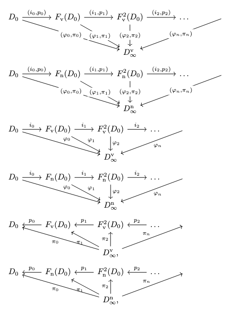
We proceed in a manner analogous to the construction of fixed points within CPOs, namely, we begin with the initial CPO \(D_0 = \{\bot\}\) and then iteratively apply \(F_{\mathrm{n}}\):

\[D_0 \xrightarrow{(i_0, p_0)} F(D_0) \xrightarrow{F_{\mathrm{n}}((i_0,p_0))} F_{\mathrm{n}}^2(D_0) \xrightarrow{F_{\mathrm{n}}^2((i_0, p_0))} \dots .\]

Here, \(i_0\) is the unique injection from \(D_0\) into \(F_{\mathrm{n}}(D_0)\) and \(p_0\) is the unique projection from \(F_{\mathrm{n}}(D_0)\) onto \(D_0\). If we consider only the injections, then we obtain a diagram in \(\mathbf{CPO}\):

\[D_0 \xrightarrow{i_0} F_{\mathrm{n}}(D_0) \xrightarrow{i_1} F_{\mathrm{n}}^2(D_0) \xrightarrow{i_2} \dots ,\]

and likewise, if we consider only the projections, then we obtain a diagram in \(\mathbf{CPO}\):

\[D_0 \xleftarrow{p_0} F_{\mathrm{n}}(D_0) \xleftarrow{p_1} F_{\mathrm{n}}^2(D_0) \xleftarrow{p_2} \dots .\]

Here, \(i_n\) and \(p_n\) satisfy \((i_n, p_n) = F_{\mathrm{n}}^n((i_0, p_0))\).

We then take the colimit of the chain of injections, which will be the fixed point we desire. Unfortunately, it is challenging to exhibit an explicit carrier of this colimit. Fortunately, however, it turns out that the colimit of the chain of injections is isomorphic to the limit of the chain of projections and it is relatively straightforward to exhibit a carrier of this limit. Furthermore, the carriers of the initial algebra and final coalgebra for the respective functor will coincide. We designate the carrier of this limit as \(D^{\mathrm{n}}_{\infty}\).

Next, we will indicate a similar construction for the call-by-value evaluation strategy.

Call-by-name requires a reflexive domain \(D \cong \mathrm{Cont}(D,D)\), whereas call-by-value naturally leads to a value domain \(V \cong \mathrm{Cont}(V, V_{\bot})\), with \(V_{\bot}\)​ serving as the computation domain.

For any CPO \(V\), we define \(V_{\bot} = V \cup \{\bot\}\) with an ordering defined as \(x \le y\) whenever \(x = \bot\) or \(x \le_V y\).

For any map \(f : D \rightarrow E\), we define \(f_{\bot} : D_{\bot} \rightarrow E_{\bot}\) as follows:

\[f_{\bot}(v) = \begin{cases}\bot & \text{if } v = \bot \\ f(v) & \text{otherwise}.\end{cases}\]

We then designate a functor \(F_{\mathrm{v}}\) on \(\mathbf{CPO}^{ep}\) as follows:

• \(F_{\mathrm{v}}(V) = \mathrm{Cont}(V, V_{\bot})\),
• \(F_{\mathrm{v}}((i, p)) = (g \mapsto i_{\bot} \circ g \circ p, h \mapsto p_{\bot} \circ h \circ i)\).

We then obtain the following diagram for \(V_0 = \{\bot\}\):

\[V_0 \xrightarrow{(i_0, p_0)} F_{\mathrm{v}}(V_0) \xrightarrow{F_{\mathrm{v}}((i_0, p_0))} F_{\mathrm{v}}^2(V_0) \xrightarrow{F_{\mathrm{v}}^2((i_0, p_0))} \dots.\]

If we consider only the injections, then we obtain a diagram in \(\mathbf{CPO}\):

\[V_0 \xrightarrow{i_0} F_{\mathrm{v}}(V_0) \xrightarrow{i_1} F_{\mathrm{v}}^2(V_0) \xrightarrow{i_2} \dots ,\]

and likewise, if we consider only the projections, then we obtain a diagram in \(\mathbf{CPO}\):

\[V_0 \xleftarrow{p_0} F_{\mathrm{v}}(V_0) \xleftarrow{p_1} F_{\mathrm{v}}^2(V_0) \xleftarrow{p_2} \dots .\]

Here, \(i_n\) and \(p_n\) satisfy \((i_n, p_n) = F_{\mathrm{v}}^n((i_0, p_0))\).

The carrier \(V\) of the inverse limit then satisfies \(F_{\mathrm{v}}(V) \cong \mathrm{Cont}(V,V_{\bot})\) and we define the carrier of the model as \(D^{\mathrm{v}}_{\infty} = V_{\bot}\).

Isomorphisms

We will define several related categories.

Definition (\(\mathbf{CPO}\)). The category \(\mathbf{CPO}\) is defined as follows:

• Objects: all pointed, directed-complete partial orders (CPOs);
• Arrows: an arrow \(f : A \rightarrow B\) is a continuous, point-preserving map (i.e., \(f(\bot_A) = \bot_B\)).

Definition (\(\mathbf{CPO}^{ep}\)). The category \(\mathbf{CPO}^{ep}\) is defined as follows:

• Objects: all pointed, directed-complete partial orders (CPOs).
• Arrows: an arrow \(\gamma : A \rightarrow B\) consists of a pair of arrows \(\gamma = (i, p)\) where \(i : A \rightarrow B\) is an arrow (called an injection) in \(\mathbf{CPO}\) and \(p : B \rightarrow A\) is an arrow (called a projection) in \(\mathbf{CPO}\) such that the following conditions are satisfied:
  • \(p \circ i = \mathrm{id}_A\);
  • \(i \circ p \le \mathrm{id}_B\).

Definition (\(\mathbf{CPO}^e\)). The category \(\mathbf{CPO}^e\) is defined as follows:

• Objects: all pointed, directed-complete partial orders (CPOs).
• Arrows: an arrow \(i : A \rightarrow B\) is an arrow \(i : A \rightarrow B\) in \(\mathbf{CPO}\) (called an injection) such that there exists an arrow \(p : B \rightarrow A\) (called a projection) in \(\mathbf{CPO}\) such that \(p \circ i = \mathrm{id}_A\).

Definition (\(\mathbf{CPO}^p\)). The category \(\mathbf{CPO}^p\) is defined as follows:

• Objects: all pointed, directed-complete partial orders (CPOs).
• Arrows: an arrow \(p : B \rightarrow A\) is an arrow \(p : B \rightarrow A\) (called a projection) in \(\mathbf{CPO}\) such that there exists an arrow \(i : A \rightarrow B\) (called an injection) in \(\mathbf{CPO}\) such that \(i \circ p \le \mathrm{id}_B\).

The difference between \(\mathbf{CPO}^{ep}\) and its counterparts \(\mathbf{CPO}^e\) and \(\mathbf{CPO}^p\), besides the structural difference in the arrows, is that arrows in \(\mathbf{CPO}^{ep}\) must satisfy two properties whereas the arrows in \(\mathbf{CPO}^e\) and \(\mathbf{CPO}^p\) must only satisfy a single property.

We will now indicate various isomorphisms between these categories.

Lemma (Isomorphism). The following strict isomorphisms of categories obtain:

• \(\mathbf{CPO}^{ep} \cong \mathbf{CPO}^e\),
• \(\mathbf{CPO}^{ep} \cong (\mathbf{CPO}^p)^{op}\).

Proof. Define a functor \(F : \mathbf{CPO}^{ep} \rightarrow \mathbf{CPO}^e\) as follows:

• \(F(A) = A\) for all objects \(A\),
• \(F(i, p) = i\) for all arrows \((i, p)\).

Define its inverse \(F^{-1} : \mathbf{CPO}^e \rightarrow \mathbf{CPO}^{ep}\) as follows:

• \(F^{-1}(A) = A\) for all objects \(A\),
• \(F^{-1}(i) = (i, p_i)\) for all arrows \(i\), where \(p_i\) is the projection corresponding to the injection \(i\).

Note that \(F(F^{-1}(i)) = i\) and \(F^{-1}(F(i,p)) = (i, p_i)\). We will now show that \(p = p_i\). Since \(i \circ p \le \mathrm{id}_B\), it follows by monotonicity that \(p_i \circ i \circ p \le p_i \circ \mathrm{id}_B\) and thus \(p \le p_i\). A symmetric argument shows that \(p_i \le p\) and thus, by antisymmetry, \(p = p_i\). Thus, projections are uniquely determined. It follows that \(F^{-1}(F)(i,p) = p\) and \(F\) and \(F^{-1}\) are mutual inverses, so there is a strict isomorphism of categories.

Define a functor \(G : \mathbf{CPO}^{ep} \rightarrow (\mathbf{CPO}^p)^{op}\) as follows:

• \(G(A) = A\) for all objects \(A\),
• \(G(i,p) = p\) for all arrows \((i,p)\).

Define its inverse \(G^{-1} : (\mathbf{CPO}^p)^{op} \rightarrow \mathbf{CPO}^{ep}\) as follows:

• \(G^{-1}(A) = A\) for all objects \(A\),
• \(G^{-1}(p) = (i_p, p)\) for all arrows \(p\), where \(i_p\) is the injection corresponding to \(p\).

Note that \(G(G^{-1})(p) = p\) and \(G^{-1}(G(i, p)) = (i_p, p)\). We will now show that \(i = i_p\). Since \(i \circ p \le \mathrm{id}_B\), it follow by monotonicity that \(i \circ p \circ i_p \le \mathrm{id}_B \circ i_p\) and thus \(i \le i_p\). A symmetric argument shows that \(i_p \le i\) and thus, by antisymmetry, \(i = i_p\). Thus, injections are uniquely determined. It follows that \(G^{-1}(G(i, p)) = (i,p)\) and \(G\) and \(G^{-1}\) are mutual inverses, so there is a strict isomorphism of categories.\(\square\)

We make the following definitions.

Definition. Given any functor \(F : \mathbf{CPO}^{ep} \rightarrow \mathbf{CPO}^{ep}\), define the following functors:

• \(F^e\):
  • Objects: \(F^e(A) = F(A)\),
  • Arrows: \(F^e(i, p) = \hat{i}\), where \(F(i, p) = (\hat{i}, \hat{p})\).
• \(F^p\):
  • Objects: \(F^p(A) = F(A)\),
  • Arrows: \(F^p(i, p) = \hat{p}\), where \(F(i, p) = (\hat{i}, \hat{p})\).

We thus have the following lemma. It follows from general facts about category theory, but we will indicate an explicit proof.

Lemma (Bilimit). Let \(J : \mathcal{D} \rightarrow \mathbf{CPO}^{ep}\) be any diagram and suppose that a co-limiting co-cone \((C, \gamma_D)_{D \in \mathcal{D}}\) (where \(\gamma_D = (i_D, p_D)\)) for \(J\) exists in \(\mathbf{CPO}^{ep}\). Then:

• A corresponding colimit \((C, i_D)_{D \in \mathcal{D}}\) for the diagram \(\mathrm{Id}^e \circ J\) exists in \(\mathbf{CPO}^e\);
• A corresponding limit \((C, p_D)_{D \in \mathcal{D}}\) for the diagram \(\mathrm{Id}^p \circ J\) exists in \(\mathbf{CPO}^p\).

Proof.

Colimits

Consider the following diagrams.

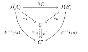
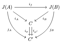
Consider any arrow \(f : A \rightarrow B\) between objects \(A,B\) in \(\mathcal{D}\). By definition of the colimit of the diagram \(J\), it follows that

\[\gamma_A = \gamma_B \circ J(f).\]

We then apply the isomorphism \(F^{-1} : \mathbf{CPO}^e \rightarrow \mathbf{CPO}^{ep}\) to obtain

\[F^{-1}(\gamma_A) = F^{-1}(\gamma_B \circ J(f)) = F^{-1}(\gamma_B) \circ F^{-1}(J(f))\]

and thus

\[i_A = i_B \circ i_f\]

where \(J(f) = (i_f, p_f)\). Thus, since \(f\) was arbitrary, \(C\) is likewise the vertex of a co-cone \((C, i_D)_{D \in \mathcal{D}}\) for the diagram \(\mathrm{Id}^e \circ J\).

Next, suppose that there exists another co-cone \((C', j_D)_{D \in \mathcal{D}}\) for the diagram \(\mathrm{Id}^e \circ J\) in \(\mathbf{CPO}^e\). Let \(f : A \rightarrow B\) be any arrow in \(\mathcal{D}\). Then, by definition,

\[j_A = j_B \circ i_f.\]

It follows that

\[F^{-1}(j_A) = F^{-1}(j_B) \circ F^{-1}(i_f) = F^{-1}(j_B) \circ J(f),\]

and thus, since \(f\) was arbitrary, \((C', F^{-1}(j_D))_{d \in \mathcal{D}}\) is a co-cone in \(\mathbf{CPO}^{ep}\) for the diagram \(J\).

Then, by the universal property of the colimit of the diagram \(J\), it follows that there exists a unique arrow \(\mu : C \rightarrow C'\) such that \(F^{-1}(j_A) = \mu \circ \gamma_A\) for every \(A \in \mathcal{D}\). Define \(i_{\mu} = F(\mu)\). It then follows that

\[F(F^{-1}(j_A)) = F(\mu \circ \gamma_A) = F(\mu) \circ F(\gamma_A) = i_{\mu} \circ i_A\]

and so \(j_A = i_{\mu} \circ i_A\). Now, suppose that there exists another arrow \(i_{\mu'} : C \rightarrow C'\) such that \(j_A = i_{\mu'} \circ i_A\). Define \(\mu' = F^{-1}(i_{\mu'})\). Then

\[F^{-1}(j_A) = F^{-1}(i_{\mu'}) \circ F^{-1}(i_B) = \mu' \circ \gamma_A\]

and thus \(F^{-1}(j_A) = \mu' \circ \gamma_B\). By the universal property of the colimit of the diagram \(J\), it follows that \(\mu' = \mu\). Then \(F(\mu') = F(\mu)\) and hence \(i_{\mu} = i_{\mu'}\) and \(i_{\mu}\) is the unique mediating arrow. Thus, the co-cone \((C, i_D)_{D \in \mathcal{D}}\) is a colimit for the diagram \(\mathrm{Id}^e \circ J\).

Limits

Consider the following diagrams.

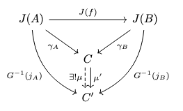
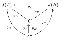
Consider any arrow \(f : A \rightarrow B\) between objects \(A,B\) in \(\mathcal{D}\). By definition of the colimit of the diagram \(J\), it follows that

\[\gamma_A = \gamma_B \circ J(f).\]

We then apply the isomorphism \(G^{-1} : (\mathbf{CPO}^p)^{op} \rightarrow \mathbf{CPO}^{ep}\) (which is contravariant as a functor \(G^{-1} : \mathbf{CPO}^p \rightarrow \mathbf{CPO}^{ep}\)) to obtain

\[G^{-1}(\gamma_A) = G^{-1}(\gamma_B \circ J(f)) = G^{-1}(J(f)) \circ G^{-1}(\gamma_B)\]

and thus

\[p_A = p_f \circ p_B.\]

Since \(f\) was arbitrary, it follows that \((C, p_D)_{D \in \mathcal{D}}\) is a cone for the diagram \(\mathrm{Id}^p \circ J\).

Next, suppose there exists another cone \((C', j_D)_{D \in \mathcal{D}}\) for the diagram \(\mathrm{Id}^p \circ J\). Let \(f : A \rightarrow B\) be any arrow in \(\mathcal{D}\). Then, by definition,

\[j_A = p_f \circ j_B.\]

It follows that

\[G^{-1}(j_A) = G^{-1}(p_f \circ j_B) = G^{-1}(j_B) \circ G^{-1}(p_f ),\]

and thus, since \(f\) was arbitrary, \((C', G^{-1}(j_D))_{D \in \mathcal{D}}\) is a co-cone for the diagram \(J\).

Then, by the universal property of the colimit for the diagram \(J\), it follows that there exists a unique arrow \(\mu : C \rightarrow C'\) in \(\mathbf{CPO}^{ep}\) such that \(G^{-1}(j_A) = \mu \circ \gamma_A\) for all objects \(A\) in \(\mathcal{D}\). Define \(p_{\mu} = G(\mu)\). Then

\[j_A = G(G^{-1}(j_A)) = G(\mu \circ \gamma_A) = G(\gamma_A) \circ G(\mu) = p_A \circ p_{\mu}.\]

Thus \(p_{\mu}\) is a mediating map. Now, suppose there exists another mediating map \(p_{\mu'} : C' \rightarrow C\) such that \(j_A = p_A \circ p_{\mu'}\). Define \(\mu' = G^{-1}(p_{\mu'})\). Then

\[G^{-1}(j_A) = G^{-1}(p_A \circ p_{\mu'}) = G^{-1}(p_{\mu'}) \circ G^{-1}(p_A) = \mu' \circ \gamma_A.\]

By the universal property of the colimit of the diagram \(J\), it follows that \(\mu = \mu'\). Then \(G(\mu) = G(\mu')\) and hence \(p_{\mu} = p_{\mu'}\) and \(p_{\mu}\) is the unique mediating map. Thus, the cone \((C, p_D)_{D \in \mathcal{D}}\) is a limit for the diagram \(\mathrm{Id}^p \circ J\). \(\square\)

The Initial Algebra Theorem

In this section, we will state and prove a general fixed point theorem for functors on categories.

Theorem (Initial Algebra). Let \(\mathbb{C}\) be any category with an initial object \(0_{\mathcal{C}}\) and colimits of all \(\omega\)-chains and \(F : \mathbb{C} \rightarrow \mathbb{C}\) be any functor that preserves all colimits of \(\omega\)-chains. Then there exists a fixed point \(\mu F\) of \(F\) that carries the initial algebra for \(F\).

Proof. The index category \(\omega\) is defined as follows:

• Objects: natural numbers \(n \in \mathbb{N}\),
• Arrows: a unique arrow \((m \le n) : m \rightarrow n\) if and only if \(m \le n\).

The diagram \(D : \omega \rightarrow \mathbb{C}\) is defined recursively as follows:

• Objects:
  • \(D(n) = 0_{\mathbb{C}}\);
  • \(D(n+1) = F(D(n))\);
• Arrows:
  • \(D(0 \le n) = i_{D(n)} : 0_{\mathbb{C}} \rightarrow D(n)\);
  • \(D(m+1 \le n+1) = F(D(m \le n))\).

Consider the following diagram for arbitrary objects \(m, n \in \omega\).

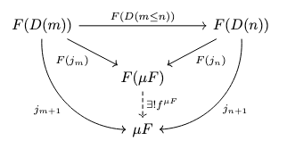
We denote the vertex of the co-cone corresponding to the diagram \(D\) as \(\mu F\) and the respective co-cone arrows are denoted as \(j_n : D(n) \rightarrow \mu F\), etc. Since \(F\) preserves directed colimits, \(F(\mu F)\) is the vertex of the co-cone corresponding to the diagram \(F \circ D\) and the respective co-cone arrows are \(F(j_n) : F(D(n)) \rightarrow F(\mu F)\), etc. Thus, by the universal property of colimits, there exists a unique arrow \(f^{\mu F} : F(\mu F) \rightarrow \mu F\) making this diagram commute. Thus, \(f^{\mu F}\) represents an algebra for the functor \(F\). Our goal is to show that it is an initial algebra.

Suppose there exists an object \(A \in \mathbb{C}\) and an arrow \(f^A : F(A) \rightarrow A\), i.e., that \(f^A\) represents an algebra for the functor \(F\). We construct a co-cone with \(A\) as its vertex recursively as follows:

• \(a_0 = i_A : 0_{\mathbb{C}} \rightarrow A\),
• \(a_{n+1} = f^A \circ F(a_n)\).

Consider the following diagram.

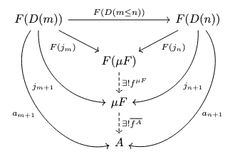
We will show by induction that the arrows \(a_n\) comprise a co-cone. First, when \(m = 0\), note that, since there is a unique arrow from \(0_{\mathbb{C}}\) to any object, it follows that

\begin{align*}a_n \circ D(0 \le n) &= a_n \circ i_{D(n)} \\&= a_0.\end{align*}

Next, suppose that \(a_n \circ D(m \le n) = a_m\) for arbitrary \(m,n \in \omega\), and consider the following:

\begin{align*}a_{n+1} \circ D(m+1 \le n+1) &= a_{n+1} \circ F(D(m \le n)) \\&= f^A \circ F(a_n) \circ F(D(m \le n)) \\&= f^A \circ F(a_n \circ D(m \le n)) \\&= f^A \circ F(a_m) \\&= a_{m+1}.\end{align*}

Thus, the arrows \(a_n\) comprise a co-cone. By the universal property of colimits, it follows that there exists a unique arrow \(\overline{f^A} : \mu F \rightarrow A\) such that the above diagram commutes.

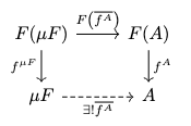
Our goal is to show that \(\mu F\) carries an initial algebra, i.e., that the following diagram commutes.

Consider the following diagram.

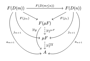
Since the co-cone for \(A\) is likewise a co-cone under the diagram \(D \circ F\), by the universal property of colimits, there exists a unique arrow \(g : F(\mu F) \rightarrow A\) making the previous diagram commute. Our goal is to show the following:

• \(g = \overline{f^A} \circ f^{\mu F}\),
• \(g = f^A \circ F\left(\overline{f^A}\right)\),

which immediately implies that the initial algebra diagram commutes. First, note the following:

\begin{align*}\overline{f^A} \circ f^{\mu F} \circ F(j_m) &= \overline{f^A} \circ j_{m+1} \\&= a_{m+1},\end{align*}

which, by the uniqueness of \(g\), implies that \(g = \overline{f^A} \circ f^{\mu F}\).

Next, note the following:

\begin{align*}f^A \circ F\left(\overline{f^A}\right) \circ F(j_m) &= f^A \circ F\left(\overline{f^A} \circ j_m\right) \\&= f^A \circ F(a_m) \\&= a_{m+1},\end{align*}

which, by the uniqueness of \(g\), implies that \(g = f^A \circ F\left(\overline{f^A}\right)\). Thus, the initial algebra diagram commutes. Finally, we need to show that \(\overline{f^A}\) is the unique arrow making the initial algebra diagram commute. Suppose there exists some arrow \(h : \mu F \rightarrow A\) such that \(h \circ f^{\mu F} = f^A \circ F(h)\). Then:

\begin{align*}h \circ j_{m+1} &= h \circ f^{\mu F} \circ F(j_m) \\&= f^A \circ F(h) \circ F(j_m) \\&= f^A \circ F(h \circ j_m) \\&= f^A \circ F(a_m) \\&= a_{m+1}.\end{align*}

Thus, by the universal property of colimits, it follows that \(h = \overline{f^A}\) and thus \(\overline{f^A}\) is unique. From this, we conclude that \(\mu F\) carries an initial algebra for \(F\).

Finally, we indicate that \(\mu F\) is a fixed point. Consider the following diagram.

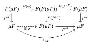
First note that, by the universal property of the initial algebra, it follows that

\[f^{\mu F} \circ \varphi = 1_{\mu F}.\]

Next, note the following:

\begin{align*}\varphi \circ f^{\mu F} &= F(f^{\mu F}) \circ F(\varphi) \\&= F(f^{\mu F} \circ \varphi) \\&= F(1_{\mu F}) = 1_{F(\mu F)}.\end{align*}

It follows that \(F(\mu F) \cong \mu F\). Thus, \(\mu F\) is a fixed point of \(F\), and it carries an initial algebra for \(F\). \(\square\)

The Characterization Lemma for Colimits

We will prove a very useful lemma in this section which characterizes directed colimits in the category \(\mathbf{CPO}^{ep}\).

Lemma (Characterization of Directed Colimits). Let \((D_n, \gamma_n)_{n \in \mathbb{N}}\) be an \(\omega\)-chain in \(\mathbf{CPO}^{ep}\), where \(\gamma_n = (i_n, p_n) : D_n \rightarrow D_{n+1}\) is an embedding-projection pair. An embedding-projection co-cone \((D, \gamma^{\infty}_n)_{n \in \mathbb{N}}\) is a colimit of the chain in \(\mathbf{CPO}^{ep}\) if and only if

\[\bigsqcup_{n=0}^{\infty}(i^{\infty}_n \circ p^{\infty}_n) = \mathrm{id}_D.\]

Proof.

Part 1: Sufficiency.

Assume \(\bigsqcup_{n=0}^{\infty}(i^{\infty}_n \circ p^{\infty}_n) = \mathrm{id}_D\). Consider the following diagram.

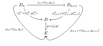
Let \((E, \mu_n)_{n \in \mathbb{N}}\) be any co-cone over \((D_n, \gamma_n)_{n \in \mathbb{N}}\), where \(\mu_n : D_n \rightarrow E\) satisfies \(\mu_{n+1} \circ \gamma_n = \mu_n\) for all \(n \in \mathbb{N}\).

Define the embedding-projection pair \((j, q) : D \rightarrow E\) as follows:

\[j = \bigsqcup_{n=0}^{\infty}(j_n \circ p^{\infty}_n),\]

\[q = \bigsqcup_{n=0}^{\infty}(i^{\infty}_n \circ q_n).\]

Properties

• Identity A: \(j \circ i^{\infty}_k = j_k\). For all \(k \in \mathbb{N}\) and \(x \in D_k\),

\begin{align*}j(i^{\infty}_k(x)) &= \bigsqcup_{n=0}^{\infty}j_n(p^{\infty}_n(i^{\infty}_k(x))) \\&= \bigsqcup_{n=k}^{\infty}j_n(p^{\infty}_n(i^{\infty}_k(x))).\end{align*}

For all \(n \ge k\), \(p^{\infty}_n \circ i^{\infty}_k = i^n_k\) and \(j_n \circ i^n_k = j_k\) (where \(i^n_k : D_k \rightarrow D_n\) is the composite map \(i^n_k = i_n \circ \dots i_k\), etc.), so we continue

\begin{align*}j(i^{\infty}_k(x)) &= \bigsqcup_{n=k}^{\infty}j_n(p^{\infty}_n(i^{\infty}_k(x))) \\&= \bigsqcup_{n=k}^{\infty}j_n( i^n_k(x)) \\&=\bigsqcup_{n=k}^{\infty}j_k(x) \\&= j_k(x).\end{align*}

• Identity B: \(q \circ j_n = i^{\infty}_n\). For any \(n \in \mathbb{N}\) and \(z \in D_n\):

\begin{align*}q(j_n(z)) &= \bigsqcup_{m=0}^{\infty}i^{\infty}_m(q_m(j_n(z))) \\&= \bigsqcup_{m=n}^{\infty}i^{\infty}_m(q_m(j_n(z))).\end{align*}

For all \(m \ge n\), \(q_m \circ j_n = p^m_n\) and \(i^{\infty}_m \circ p^m_n = i^{\infty}_n\), so we continue

\begin{align*}q(j_n(z)) &= \bigsqcup_{m=n}^{\infty}i^{\infty}_m(q_m(j_n(z))) \\&= \bigsqcup_{m=n}^{\infty}i^{\infty}_m(p^m_n(z))) \\&= \bigsqcup_{m=n}^{\infty} i^{\infty}_n(z) \\&= i^{\infty}_n(z).\end{align*}

Embedding-Projection Pair Verification

• \(q \circ j = \mathrm{id}_D\): We apply Identity B and exploit the continuity of \(q\):

\begin{align*}q(j(x)) &= q\left(\bigsqcup_{n=0}^{\infty} j_n(p^{\infty}_n(x))\right) \\&= \bigsqcup_{n=0}^{\infty} q(j_n(p^{\infty}_n(x))) \\&= \bigsqcup_{n=0}^{\infty}i^{\infty}_n(p^{\infty}_n(x)) \\&= \mathrm{id}_D(x).\end{align*}

• \(j \circ q \le \mathrm{id}_E\). We apply Identity B and exploit the continuity of \(j\):

\begin{align*}j(q(y)) &= j\left(\bigsqcup_{m=0}^{\infty}i^{\infty}_m(q_m(y))\right) \\&= \bigsqcup_{m=0}^{\infty}j(i^{\infty}_m(q_m(y))) \\&= \bigsqcup_{m=0}^{\infty}j_m(q_m(y)) \\&\le \bigsqcup_{m=0}^{\infty}\mathrm{id}_E(y) \\&= y.\end{align*}

Commutativity and Uniqueness

• Commutativity: (\(\mu \circ \gamma^{\infty}_k = \mu_k\)). Note that \(j \circ i^{\infty}_k = j_k\) holds by Identity A. Also, note that

\begin{align*}p^{\infty}_k(q(y)) &= \bigsqcup_{m=0}^{\infty} p^{\infty}_k(i^{\infty}_m(q_m(y))) \\&= \bigsqcup_{m=k}^{\infty} p^{\infty}_k(i^{\infty}_m(q_m(y))) \\&= \bigsqcup_{m=k}^{\infty} i^m_k(q_m(y)) \\&= q_k(y).\end{align*}

• Uniqueness: if \(\mu' = (j', q')\) satisfies \(\mu' \circ \gamma^{\infty}_n = \mu_n\) for all \(n \in \mathbb{N}\), then

\begin{align*}j'(x) &= j'\left( \bigsqcup_{n=0}^\infty i_n^\infty(p_n^\infty(x)) \right) \\&= \bigsqcup_{n=0}^\infty j'(i_n^\infty(p_n^\infty(x))) \\&= \bigsqcup_{n=0}^\infty j_n(p_n^\infty(x)) \\&= j(x),\end{align*}

and similarly, \(q' = q\), so \(\mu' = \mu\) and \(\mu\) is unique.

Part 2: Necessity.

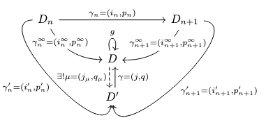
Suppose \((D, \gamma^{\infty}_n)_{n \in \mathbb{N}}\) is a colimit of \((D_n, \gamma_n)_{n \in \mathbb{N}}\) in \(\mathbf{CPO}^{ep}\). Define \(g : D \rightarrow D\) as

\[g = \bigsqcup_{n=0}^{\infty}(i^{\infty}_n \circ p^{\infty}_n).\]

Since \(i^{\infty}_n \circ p^{\infty}_n \le \mathrm{id}_D\) for all \(n \in \mathbb{N}\), it follows that \(g \le \mathrm{id}_D\).

• Idempotence: (\(g \circ g = g\)). Note that

\begin{align*}p^{\infty}_n(g(x)) &= p^{\infty}_n\left(\bigsqcup_{m=0}^{\infty}i^{\infty}_m( p^{\infty}_m(x))\right) \\&= \bigsqcup_{m=0}^{\infty}p^{\infty}_n(i^{\infty}_m( p^{\infty}_m(x)) \\&= \bigsqcup_{m=n}^{\infty}p^{\infty}_n(i^{\infty}_m( p^{\infty}_m(x)) \\&= \bigsqcup_{m=n}^{\infty}p^n_m(p^{\infty}_m(x)) \\&= p^{\infty}_n(x)\end{align*}

and therefore

\begin{align*}g(g(x)) &= \bigsqcup_{n=0}^{\infty}i^{\infty}_n(p^{\infty}_n(g(x))) \\&= \bigsqcup_{n=0}^{\infty}i^{\infty}_n(p^{\infty}_n(x)) \\&= g(x).\end{align*}

• Fixed Point CPO: We define a sub-CPO consisting of the fixed points of \(g\) as follows:

\[D' = \{x \in D \mid g(x) = x\}.\]

The inclusion \(j : D' \rightarrow D\) and the restriction \(q = g \vert^{D'}_{D} : D \rightarrow D'\) form an embedding-projection pair \(\gamma = (j,q) : D' \rightarrow D\) with \(j \circ q = g\).

• Co-cone: Because \(g(i^{\infty}_n(x)) = i^{\infty}_n(x)\), it follows that \(i^{\infty}_n(x) \in D'\) for all \(x \in D\), and hence we define \(i'_n : D_n \rightarrow D'\) as \(i'_n = i^{\infty}_n \vert_{D_n}^{D'}\) for all \(n \in \mathbb{N}\). We likewise define \(p'_n = p^{\infty}_n \circ j\) for all \(n \in \mathbb{N}\). Thus, we define \(\gamma'_n = (i'_n, p'_n)\) for all \(n \in \mathbb{N}\) and \(D', \gamma'_n)_{n \in \mathbb{N}}\) is an embedding-projection co-cone over \((D_n, \gamma_n)_{n \in \mathbb{N}}\).
• Universal Property: By the universal property of \((D_n, \gamma_n)_{n \in \mathbb{N}}\), there exists a unique mediating map \(\mu = (j_{\mu}, q_{\mu}) : D \rightarrow D'\) such that \(\mu \circ \gamma^{\infty}_n = \gamma'_n\). The composite \(\gamma \circ \mu : D \rightarrow D\) satisfies

\begin{align*}(\gamma \circ \mu) \circ \gamma^{\infty}_n &= \gamma \circ \gamma'_n \\&= (j \circ i'_n, p'_n \circ q) \\&= (i^{\infty}_n, p^{\infty}_n \circ j \circ q) \\&= (i^{\infty}_n, p^{\infty}_n \circ g) \\&= (i^{\infty}_n, p^{\infty}_n) \\&= \gamma^{\infty}_n.\end{align*}

By the uniqueness of mediating maps for colimits, it follows that \(\gamma \circ \mu = (\mathrm{id}_D, \mathrm{id}_D)\), which implies that \(j \circ j_{\mu} = \mathrm{id}_D\). Since \(j : D' \rightarrow D\) is an inclusion map, it follows that \(D = D'\) and hence \(g = \mathrm{id}_D\). \(\square\)

Local Continuity

Next, we will describe local continuity and prove an important lemma.

Definition (Locally Continuous Functor). A functor \(F : \mathbf{CPO}^{ep} \rightarrow \mathbf{CPO}^{ep}\) is locally continuous if the maps

\[F_{A,B} : \mathrm{Hom}(A, B) \rightarrow \mathrm{Hom}(F(A), F(B))\]

where \(F_{A,B} = \gamma \mapsto F(\gamma)\) are continuous for every \(A,B \in \mathbf{CPO}^{ep}\) with respect to the ordering

\[\gamma_1 \le \gamma_2 \Leftrightarrow i_1 \le i_2 \text{( or, equivalently \(p_1 \ge p_2\))},\]

where \(\gamma_1 = (i_1, p_1)\) and \(\gamma_2 = (i_2, p_2)\).

We have the following lemma.

Lemma (Local Continuity). If a functor \(F : \mathbf{CPO}^{ep} \rightarrow \mathbf{CPO}^{ep}\) is locally continuous, then \(F\) preserves all colimits of \(\omega\)-chains.

Proof. Let \((D_n \gamma_n)_{n \in \mathbb{N}}\) be an \(\omega\)-chain in \(\mathbf{CPO}^{ep}\) with colimit \((D, \gamma^{\infty}_n)_{n \in \mathbb{N}}\), where \(\gamma_n = (i_n, p_n)\) and \(\gamma^{\infty}_n = (i^{\infty}_n, p^{\infty}_n)\). By the characterization lemma, it follows that

\[\bigsqcup_{n=0}^{\infty}(i^{\infty}_n \circ p^{\infty}_n) = \mathrm{id}_D.\]

Note that

\begin{align*}\mathrm{id}_{F(D)} &= F(\mathrm{id}_D) \\&= F \left(\bigsqcup_{n=0}^{\infty}(i^{\infty}_n \circ p^{\infty}_n)\right) \\&= \bigsqcup_{n=0}^{\infty}F(i^{\infty}_n \circ p^{\infty}_n) & \text{(by continuity of \(F_{D,D}\))} \\&= \bigsqcup_{n=0}^{\infty}(F(i^{\infty}_n) \circ F(p^{\infty}_n)).\end{align*}

Thus, it follows that

\[\bigsqcup_{n=0}^{\infty}(F(i^{\infty}_n) \circ F(p^{\infty}_n)) = \mathrm{id}_{F(D)}\]

which, by the characterization lemma, implies that the co-cone \((F(D), \gamma^{\infty}_n)_{n \in \mathbb{N}}\) is a colimit for the \(\omega\)-chain \((F(D_n), F(\gamma_n))_{n \in \mathbb{N}}\). Thus, \(F\) preserves the colimit of the chain \((D_n, \gamma_n)_{n \in \mathbb{N}}\). \(\square\)

We will now establish that the functors \(F_{\mathrm{n}}\) and \(F_{\mathrm{v}}\) are locally continuous.

Theorem (\(F_{\mathrm{n}}\) locally continuous). The functor \(F_{\mathrm{n}}\) is well-defined and locally continuous.

Proof. Recall that \(F_{\mathrm{n}} : \mathbf{CPO}^{ep} \rightarrow \mathbf{CPO}^{ep}\) is defined as follows:

• Objects: \(F_{\mathrm{n}}(D) = D^D\), i.e., the exponential object \(\mathrm{Cont}(D,D)\) of continuous maps on \(D\) ordered pointwise, i.e., \(f \le g \Leftrightarrow \forall x \in D(f(x) \le g(x))\);
• Arrows: For \(\gamma = (i,p) : D \rightarrow E\), \(F_{\mathrm{n}}(\gamma) = (\hat{i}, \hat{p})\), where
  • \(\hat{i}(f) = i \circ f \circ p\),
  • \(\hat{p}(g) = p \circ g \circ i\).

We first confirm that \(F\) is well-defined. Note that, for any \(f \in D^D\),

\begin{align*}\hat{p}(\hat{i}(f)) &= p \circ (i \circ f \circ p) \circ i \\&= (p \circ i) \circ f \circ (p \circ i) \\&= \mathrm{id} \circ f \circ \mathrm{id} \\&= f,\end{align*}

and hence \(\hat{p} \circ \hat{i} = \mathrm{id}_{F(D)}.\) Next, note that, for any \(g \in E^E\),

\begin{align*}\hat{i}(\hat{p}(g)) &= i \circ (p \circ g \circ i) \circ p \\&= (i \circ p) \circ g \circ (i \circ p) \\&\le \mathrm{id}_E \circ g \circ \mathrm{id}_E \\&= g,\end{align*}

and hence \(\hat{i} \circ \hat{p} \le \mathrm{id}_E\). It follows that \(F(\gamma) = (\hat{i}, \hat{p})\) is an embedding-projection pair.

Next, note that for \(\mathrm{id}_D = (\mathrm{id}_D, \mathrm{id}_D)\),

\[\hat{\mathrm{id}_D}(f) = \mathrm{id}_D \circ f \circ \mathrm{id}_D = f = \mathrm{id}_{F(D)}(f),\]

and hence \(F(\mathrm{id}_D) = \mathrm{id}_{F(D)}\). For \(\gamma_1 = (i_1, p_1) : A \rightarrow B\) and \(\gamma_2 = (i_2, p_2) : B \rightarrow C\), note that, for any \(f : A \rightarrow A\),

\begin{align*}\widehat{i_2 \circ i_1}(f) &= (i_2 \circ i_1) \circ f \circ (p_2 \circ p_1) \\&= i_2 \circ (i_1 \circ f \circ p_2) \circ p_1 \\&= i_2 \circ \hat{i_1}(f) \circ p_1 \\&= \hat{i_2}(\hat{i_1}(f)) \\&= (\hat{i_2} \circ \hat{i_1})(f),\end{align*}

and, for any \(g : C \rightarrow C\),

\begin{align*}\widehat{p_1 \circ p_2}(g) &= (p_1 \circ p_2) \circ g \circ (i_2 \circ i_1) \\&= p_1 \circ (p_2 \circ g \circ i_2) \circ i_1 \\&= p_1 \circ \hat{p_2}(g) \circ i_1 \\&= \hat{p_1}(\hat{p_2}(g)) \\&= (\hat{p_1} \circ \hat{p_2})(g),\end{align*}

and hence \(F(\gamma_2 \circ \gamma_1) = F(\gamma_2) \circ F(\gamma_1)\). Thus, we have confirmed that \(F\) is a well-defined functor.

Let \((\gamma_{\alpha})_{\alpha \in A} = (i_{\alpha}, p_{\alpha})_{\alpha \in A}\) be a directed family of embedding-projection pairs in \(\mathbf{CPO}^{ep}(D, E)\) with supremum \(\bigsqcup_{\alpha \in A}\gamma_{\alpha} = \gamma = (i,p)\) where \(i = \bigsqcup_{\alpha \in A}i_{\alpha}\). Note that, for any \(f \in D^D\) and \(y \in E\),

\begin{align*}\left(\bigsqcup_{\alpha \in A}\hat{i_{\alpha}}\right)(f)(y) &= \bigsqcup_{\alpha \in A}\hat{i_{\alpha}}(f)(y) & \text{(pointwise suprema)} \\&= \bigsqcup_{\alpha \in A}(i_{\alpha} \circ f \circ p_{\alpha})(y) \\&= \bigsqcup_{\alpha \in A}i_{\alpha}(f(p_{\alpha}(y))) \\&\le \bigsqcup_{\alpha \in A}i_{\alpha}\left(f\left(\bigsqcup_{\alpha \in A}p_{\alpha}(y)\right)\right) & \text{(monotonicity)} \\&= \left(\bigsqcup_{\alpha \in A}i_{\alpha}\right)f\left(\bigsqcup_{\alpha \in A}p_{\alpha}(y)\right) & \text{(pointwise suprema)} \\&= i(f(p(y))) \\&= \hat{i}(f)(y).\end{align*}

Thus, we conclude by the definition of ordering on \(\mathbf{CPO}^{ep}(D, E)\) that

\[\bigsqcup_{\alpha \in A}F_{\mathrm{n}}(\gamma_{\alpha}) \le F_{\mathrm{n}}\left(\bigsqcup_{\alpha \in A}\gamma_{\alpha}\right).\]

In \(\mathbf{CPO}^{ep}\), \(\gamma_{\alpha} \le \gamma\) implies \(p \le p_{\alpha}\) for all \(\alpha \in A\). Thus, by monotonicity, it follows that

\begin{align*}\hat{i}(f)(y) &= i(f(p(y))) \\&= \left(\bigsqcup_{\alpha \in A}i_{\alpha}\right)(f(p(y))) \\&= \bigsqcup_{\alpha \in A}i_{\alpha}(f(p(y))) & \text{(pointwise suprema)} \\&\le \bigsqcup_{\alpha \in A}i_{\alpha}(f(p_{\alpha}(y))) \\&= \left(\bigsqcup_{\alpha \in A}\hat{i_{\alpha}}\right)(f)(y).\end{align*}

Thus, we conclude by the definition of ordering on \(\mathbf{CPO}^{ep}(D, E)\) that

\[F_{\mathrm{n}}\left(\bigsqcup_{\alpha \in A}\gamma_{\alpha}\right) \le \bigsqcup_{\alpha \in A}F_{\mathrm{n}}(\gamma_{\alpha}).\]

By antisymmetry, it follows that

\[F_{\mathrm{n}}\left(\bigsqcup_{\alpha \in A}\gamma_{\alpha}\right) = \bigsqcup_{\alpha \in A}F_{\mathrm{n}}(\gamma_{\alpha}),\]

and thus \(F_{\mathrm{n}}\) is locally continuous. \(\square\)

Theorem (\(F_{\mathrm{v}}\) locally continuous). The functor \(F_{\mathrm{v}}\) is well-defined and locally continuous.

Proof. Recall that \(F_{\mathrm{v}} : \mathbf{CPO}^{ep} \rightarrow \mathbf{CPO}^{ep}\) is defined as follows:

• Objects: \(F_{\mathrm{v}}(V) = \mathrm{Cont}(V, V_{\bot})\), i.e., the exponential object \(\mathrm{Cont}(V,V_{\bot})\) of continuous maps from \(V\) to \(V_{\bot}\) (where \(V_{\bot} = V \cup \{\bot_{\bot}\}\) adds a fresh bottom element \(\bot_{\bot}\) below all elements of \(V\)) ordered pointwise, i.e., \(f \le g \Leftrightarrow \forall x \in V(f(x) \le g(x))\);
• Arrows: For \(\gamma = (i,p) : V \rightarrow W\), \(F_{\mathrm{v}}(\gamma) = (\hat{i}, \hat{p}) \in \mathbf{CPO}^{ep}(\mathrm{Cont}(V, V_{\bot}),\mathrm{Cont}(W, W_{\bot}))\), where
  • \(\hat{i}(f) = i_{\bot} \circ f \circ p\),
  • \(\hat{p}(g) = p_{\bot} \circ g \circ i\),
  • \(i_{\bot}(v) = \begin{cases}\bot_{\bot} & \text{ if } v = \bot_{\bot} \\ i(v) & \text{ if } v \in V,\end{cases}\)
  • \(p_{\bot}(v) = \begin{cases}\bot_{\bot} & \text{ if } v = \bot_{\bot} \\ p(v) & \text{ if } v \in V.\end{cases}\)

We first confirm that \(F\) is well-defined. Note that, for any \(f \in \mathrm{Cont}(V, V_{\bot})\),

\begin{align*}\hat{p}(\hat{i}(f)) &= p_{\bot} \circ (i_{\bot} \circ f \circ p) \circ i \\&= (p_{\bot} \circ i_{\bot}) \circ f \circ (p \circ i) \\&= \mathrm{id}_{V_{\bot}} \circ f \circ \mathrm{id}_V \\&= f,\end{align*}

and hence \(\hat{p} \circ \hat{i} = \mathrm{id}_{F(V)}.\) Next, note that, for any \(g \in W^{W_{\bot}}\),

\begin{align*}\hat{i}(\hat{p}(g)) &= i_{\bot} \circ (p_{\bot} \circ g \circ i) \circ p \\&= (i_{\bot} \circ p_{\bot}) \circ g \circ (i \circ p) \\&\le \mathrm{id}_{W_{\bot}} \circ g \circ \mathrm{id}_W \\&= g,\end{align*}

and hence \(\hat{i} \circ \hat{p} \le \mathrm{id}_W\). It follows that \(F(\gamma) = (\hat{i}, \hat{p})\) is an embedding-projection pair.

Next, note that for \(\mathrm{id}_V = (\mathrm{id}_V, \mathrm{id}_V)\),

\[\hat{\mathrm{id}_V}(f) = (\mathrm{id}_V)_{\bot} \circ f \circ \mathrm{id}_V = f = \mathrm{id}_{F(V)}(f),\]

and hence \(F(\mathrm{id}_V) = \mathrm{id}_{F(V)}\). For \(\gamma_1 = (i_1, p_1) : A \rightarrow B\) and \(\gamma_2 = (i_2, p_2) : B \rightarrow C\), note that, for any \(f : A \rightarrow A\),

\begin{align*}\widehat{i_2 \circ i_1}(f) &= (i_2 \circ i_1)_{\bot} \circ f \circ (p_2 \circ p_1) \\&= (i_2)_{\bot} \circ ((i_1)_{\bot} \circ f \circ p_2) \circ p_1 \\&= (i_2)_{\bot} \circ \hat{i_1}(f) \circ p_1 \\&= \hat{i_2}(\hat{i_1}(f)) \\&= (\hat{i_2} \circ \hat{i_1})(f),\end{align*}

and, for any \(g : C \rightarrow C\),

\begin{align*}\widehat{p_1 \circ p_2}(g) &= (p_1 \circ p_2)_{\bot} \circ g \circ (i_2 \circ i_1) \\&= (p_1)_{\bot} \circ ((p_2)_{\bot} \circ g \circ i_2) \circ i_1 \\&= (p_1)_{\bot} \circ \hat{p_2}(g) \circ i_1 \\&= \hat{p_1}(\hat{p_2}(g)) \\&= (\hat{p_1} \circ \hat{p_2})(g),\end{align*}

and hence \(F(\gamma_2 \circ \gamma_1) = F(\gamma_2) \circ F(\gamma_1)\). Thus, we have confirmed that \(F\) is a well-defined functor.

Next, we introduce a lifting construct

\[(\cdot)_{\bot} : \mathbf{CPO}^{ep}(V, W) \rightarrow \mathbf{CPO}^{ep}(V_{\bot}, W_{\bot})\]

defined as follows:

\[(i, p)_{\bot} = (i_{\bot}, p_{\bot}).\]

We first confirm that this lifting is continuous. Let \((i_{\alpha})_{\alpha \in A}\) be a directed family of embeddings in \(\mathbf{CPO}^{ep}(V,W)\) with supremum \(i = \bigsqcup_{\alpha \in A}i_{\alpha}\). Then:

• for \(x = \bot_{\bot}\):

\begin{align*}\left(\bigsqcup_{\alpha \in A}i_{\alpha}\right)_{\bot}\left(\bot_{\bot}\right) &= \bot_{\bot} \\&= \bigsqcup_{\alpha \in A}\bot_{\bot} \\&= \bigsqcup_{\alpha \in A}\left((i_{\alpha})_{\bot}\left(\bot_{\bot}\right)\right);\end{align*}

• for \(x = v \in V\):

\begin{align*}\left(\bigsqcup_{\alpha \in A}i_{\alpha}\right)_{\bot}(v) &= \left(\bigsqcup_{\alpha \in A}i_{\alpha}\right)(v) \\&= \bigsqcup_{\alpha \in A}(i_{\alpha}(v)) \\&= \bigsqcup_{\alpha \in A}((i_{\alpha})_{\bot}(v)) .\end{align*}

Let \((\gamma_{\alpha})_{\alpha \in A} = (i_{\alpha}, p_{\alpha})_{\alpha \in A}\) be a directed family of embedding-projection pairs in \(\mathbf{CPO}^{ep}(V, W)\) with supremum \(\bigsqcup_{\alpha \in A}\gamma_{\alpha} = \gamma = (i,p)\) where \(i = \bigsqcup_{\alpha \in A}i_{\alpha}\). Note that, for any \(f \in \mathrm{Cont}(V, V_{\bot})\) and \(w \in W\),

\begin{align*}\left(\bigsqcup_{\alpha \in A}\hat{i_{\alpha}}\right)(f)(w) &= \bigsqcup_{\alpha \in A}\hat{i_{\alpha}}(f)(w) & \text{(pointwise suprema)} \\&= \bigsqcup_{\alpha \in A}((i_{\alpha})_{\bot} \circ f \circ p_{\alpha})(w) \\&= \bigsqcup_{\alpha \in A}(i_{\alpha})_{\bot}(f(p_{\alpha}(w))) \\&\le \bigsqcup_{\alpha \in A}(i_{\alpha})_{\bot}\left(f\left(\bigsqcup_{\alpha \in A}p_{\alpha}(w)\right)\right) & \text{(monotonicity)} \\&= \left(\bigsqcup_{\alpha \in A}(i_{\alpha})_{\bot}\right)f\left(\bigsqcup_{\alpha \in A}p_{\alpha}(w)\right) & \text{(pointwise suprema)} \\&= i_{\bot}(f(p(w))) \\&= \hat{i}(f)(w).\end{align*}

Thus, we conclude by the definition of ordering on \(\mathbf{CPO}^{ep}(V, W)\) that

\[\bigsqcup_{\alpha \in A}F_{\mathrm{v}}(\gamma_{\alpha}) \le F_{\mathrm{v}}\left(\bigsqcup_{\alpha \in A}\gamma_{\alpha}\right).\]

In \(\mathbf{CPO}^{ep}\), \(\gamma_{\alpha} \le \gamma\) implies \(p \le p_{\alpha}\) for all \(\alpha \in A\). Thus, by monotonicity, it follows that

\begin{align*}\hat{i}(f)(w) &= i_{\bot}(f(p(y))) \\&= \left(\bigsqcup_{\alpha \in A}(i_{\alpha})_{\bot}\right)(f(p(w))) \\&= \bigsqcup_{\alpha \in A}(i_{\alpha})_{\bot}(f(p(w))) & \text{(pointwise suprema)} \\&\le \bigsqcup_{\alpha \in A}(i_{\alpha})_{\bot}(f(p_{\alpha}(w))) \\&= \left(\bigsqcup_{\alpha \in A}\hat{i_{\alpha}}\right)(f)(w).\end{align*}

Thus, we conclude by the definition of ordering on \(\mathbf{CPO}^{ep}(V, W)\) that

\[F_{\mathrm{v}}\left(\bigsqcup_{\alpha \in A}\gamma_{\alpha}\right) \le \bigsqcup_{\alpha \in A}F_{\mathrm{v}}(\gamma_{\alpha}).\]

By antisymmetry, it follows that

\[F_{\mathrm{v}}\left(\bigsqcup_{\alpha \in A}\gamma_{\alpha}\right) = \bigsqcup_{\alpha \in A}F_{\mathrm{v}}(\gamma_{\alpha}),\]

and thus \(F_{\mathrm{v}}\) is locally continuous. \(\square\)

Construction of Colimits

We will begin by exhibiting the construction of colimits of \(\omega\)-chains in \(\mathbf{CPO}^{ep}\).

Let \((X_n)_{n \in \mathbb{N}}\) be any sequence of pointed, directed-complete partial orders (CPOs). For each \(n \in \mathbb{N}\), let \((i_n, p_n)\) be a pair of continuous maps \(i_n : X_n \rightarrow X_{n+1}\) and \(p_n : X_{n+1} \rightarrow X_n\) satisfying the following properties:

• \(p_n \circ i_n = \mathrm{id}_{X_n}\),
• \(i_n \circ p_n \le \mathrm{id}_{X_{n+1}}\).

Note that both the call-by-name functor \(F\) and the call-by-value functor \(F_{\bot}\) generate sequences satisfying these conditions.

We define the carrier \(X_{\infty}\) as the set of all coherent sequences, namely, as the following set:

\[X_{\infty} = \left\{x \in \prod_{n \in \mathbb{N}}X_n ~\middle|~ \forall n \in \mathbb{N}(x_n = p_n(x_{n+1}))\right\}.\]

We equip \(X_{\infty}\) with a pointwise ordering defined as follows:

\[x \le y \Leftrightarrow \forall n \in \mathbb{N}(x_n \le_{X_n} y_n).\]

Note that, since \((X_n, \le_{X_n})\) is a partial order for every \(n \in \mathbb{N}\), the pointwise ordering is likewise a partial order.

Next, we consider the suprema of directed subsets. Let \(Y \subseteq X_{\infty}\) be any directed subset. We will verify that the supremum of \(Y\) is as follows:

\[\left(\bigsqcup Y\right)_n = \bigsqcup Y_n = \bigsqcup_{y \in Y}y_n\]

where

\[Y_n = \{y_n \in X_n \mid y \in Y\}.\]

Note that \(Y_n\) is indeed a directed subset of \(X_n\) since the map \(\pi_n : X_{\infty} \rightarrow X_n\) defined as \(\pi_n(y) = y_n\) is monotone, so, if \(x_n, y_n \in Y_n\) then \(x,y \in Y\) and hence, since \(Y\) is a directed subset, there exists some \(z \in Y\) such that \(x \le z\) and \(y \le z\) and thus \(x_n = \pi_n(x) \le \pi_n(z) = z_n\) and \(y_n = \pi_n(y) \le \pi_n(z) = z_n\).

Next, we verify that \(\bigsqcup Y \in X_{\infty}\). By the continuity of each projection map, and, since each element of \(Y\) is coherent, it follows that

\begin{align*}p_n\left(\left(\bigsqcup Y\right)_{n+1}\right) &= p_n\left(\bigsqcup_{y \in Y} y_{n+1}\right) \\&= \bigsqcup_{y \in Y}p_n(y_{n+1}) \\&= \bigsqcup_{y \in Y}y_n \\&= \left(\bigsqcup Y\right)_n.\end{align*}

Thus \(\bigsqcup Y\) is coherent and hence \(\bigsqcup Y \in X_{\infty}\).

Next, we will verify that \(\bigsqcup Y\) is an upper bound of \(Y\). For any element \(y \in Y\), \(y_n \le \bigsqcup Y_n = \left(\bigsqcup Y\right)_n\), so \(y \le \bigsqcup Y\) and \(\bigsqcup Y\) is indeed an upper bound. For any other upper bound \(z\) of \(Y\), \(\left(\bigsqcup Y\right)_n = \bigsqcup Y_n \le z_n\) since \(z_n\) is an upper bound of \(Y_n\), so \(\bigsqcup Y \le z\) and \(\bigsqcup Y\) is the least upper bound of \(Y\).

Next, we define the bottom element of \(X_{\infty}\) as

\[\left(\bot_{X_{\infty}}\right)_n = \bot_{X_n}.\]

First, we check that \(\bot_{X_{\infty}}\) is coherent. For all \(n \in \mathbb{N}\), since \(\bot_{X_{n+1}}\) is the least element of \(X_{n+1}\), it follows that \(\bot_{X_{n+1}} \le i(\bot_{X_n})\). Since \(p_n\) is continuous, it is monotone, and hence \(p_n(\bot_{X_{n+1}}) \le p_n(i_n(\bot_{X_n}))\). Since \(p_n \circ i_n = \mathrm{id}_{X_n}\), it follows that \(p_n(\bot_{X_{n+1}}) \le \bot_{X_n}\). Since \(\bot_{X_n}\) is the least element of \(X_n\), it follows that \(\bot_{X_n} \le p_n(\bot_{X_{n+1}})\). Then, by anti-symmetry, it follows that \(p_n(\bot_{X_{n+1}}) = \bot_{X_n}\), and hence \(\bot_{X_{\infty}}\) is coherent and \(\bot_{X_{\infty}} \in X_{\infty}\).

Furthermore, for any \(x \in X_{\infty}\), \(\left(\bot_{X_{\infty}}\right)_n = \bot_{X_n} \le x_n\), so \(\bot_{X_{\infty}} \le x\) and \(\bot_{X_{\infty}}\) is the least element of \(X_{\infty}\).

Thus, we have confirmed that \(X_{\infty}\) is indeed a pointed, directed-complete partial order (CPO).

Next, we define canonical maps \(\varphi_n : X_n \rightarrow X_{\infty}\). Note that, for \(x_n \in X_n\), it must be the case that \(p_{n-1}(x_n) = x_{n-1}\) and likewise that \(p_{n-2}(x_{n-1}) = x_{n-2}\) and thus \(x_{n-2} = (p_{n-2} \circ p_{n-1})(x_n)\), etc. Likewise, it must be the case that \(p_n(x_{n+1}) = x_n\) which will be satisfied if \(x_{n+1} = i_n(x_n)\) since \(p_n(i_n(x_n)) = x_n\) and also \(x_{n+2}\) will satisfy \(p_{n+1}(x_{n+2}) = x_{n+1}\) if \(x_{n+2} = (i_{n+1} \circ i_n)(x_n)\). Thus, we make the following definition:

\[\varphi_n(x) = (y_k)_{k \in \mathbb{N}}\]

where

\[y_k = \begin{cases}(p_k \circ p_{k+1} \circ \dots \circ p_{n-1})(x) & \text{if } k \lt n \\ x & \text{if } k = n \\ (i_{k-1} \circ i_{k-2} \circ \dots \circ i_{n})(x) & \text{if } k \gt n.\end{cases}\]

First, we confirm that this is indeed a valid map \(\varphi_n : X_n \rightarrow X_{\infty}\), i.e., we verify that \(\varphi_n(x) \in X_{\infty}\) for all \(x \in X_n\) and \(n \in \mathbb{N}\). We need to show that \(p_k(y_{k+1}) = y_k\) for all \(k \in \mathbb{N}\).

• Case 1 (\(k+1 \lt n\)):

\[p_k(y_{k+1}) = p_k((p_{k+1} \circ \dots \circ p_{n-1})(x)) = (p_k \circ p_{k+1} \circ \dots \circ p_{n-1})(x) = y_k;\]

• Case 2 (\(k+1 = n\)):

\[p_k(y_{k+1}) = p_{n-1}(y_n) = p_{n-1}(x) = y_{n-1} = y_k;\]

• Case 3 (\(k+1 \gt n\)):

\[p_k(y_{k+1}) = p_k((i_k \circ i_{k-1} \circ \dots \circ i_n)(x)) = (i_{k-1} \circ \dots \circ i_n)(x) = y_k.\]

Next, we define canonical projections \(\pi_n : X_{\infty} \rightarrow X_n\) as follows:

\[\pi_n(x) = x_n.\]

We need to confirm that the pair \((\varphi_n, \pi_n)\) represents an embedding-projection pair for every \(n \in \mathbb{N}\). Note that, \((\pi_n \circ \varphi_n)(x) = x\) so \(\pi_n \circ \varphi_n = \mathrm{id}_{X_n}\).

Next, we will show that \(\varphi_n \circ \pi_n \le \mathrm{id}_{X_{\infty}}\), i.e., that \(\varphi_n(\pi_n(x)) \le x\) for all \(x \in X_{\infty}\), which means we must show that \(y_k \le x_k\) for all \(k \in \mathbb{N}\), where \(y_k = \varphi_n(x_n)\).

• Case 1 (\(k \lt n\)): \(y_k = (p_k \circ \dots \circ p_{n-1})(x_n)\) and thus \(y_k = x_k\) since \(x_{n-1} = p_{n-1}(x_n)\) and \(x_{n-2} = p_{n-2}(x_{n-1}) = (p_{n-2} \circ p_{n-1})(x_n)\), etc., so \(x_k = (p_k \circ \dots \circ p_{n-1})(x_n) = y_k\).
• Case 2 (\(k = n\)): \(y_k = x_n = x_k\).
• Case 3 (\(k \gt n\)): \(y_k = (i_{k-1} \circ \dots \circ i_n)(x_n)\) and, since \(i_n(x_n) = i_n(p_n(x_{n+1})) \le x_{n+1}\), it follows by induction that and so \(y_k = (i_{k-1} \circ \dots \circ i_n)(x_n) \le x_k\).

Next, we will confirm commutativity, namely, that \((\varphi_{n+1}, \pi_{n+1}) \circ (i_n, p_n) = (\varphi_n, \pi_n)\), which means that \(\varphi_{n+1} \circ i_n = \varphi_n\) and \(p_n \circ \pi_{n+1} = \pi_n\).

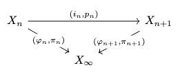
• \(\varphi_{n+1} \circ i_n = \varphi_n\): let \(y_k = \varphi_{n+1}(i_n(x))\) and \(z_k = \varphi_n(x)\);
  • Case 1 (\(k \lt n+1\)):
    • Case 1a (\(k \lt n\)): then \(y_k = (p_k \circ \dots \circ p_n)(i_n(x)) = (p_k \circ \dots \circ p_{n-1})(x) = z_k\);
    • Case 1b (\(k = n\)): then \(y_k = p_n(i_n(x)) = x = z_k\);
  • Case 2 (\(k = n+1\)): then \(y_k = i_n(x)\) and, since \(k \gt n\), \(z_k = i_n(x) = y_k\);
  • Case 3 (\(k \gt n+1\)): then \(y_k = (i_{k-1} \circ \dots \circ i_{n+1})(i_n(x)) = (i_{k-1} \circ \dots \circ i_n)(x) = z_k\) (since \(k \gt n\)\).
• \(p_n \circ \pi_{n+1} = \pi_n\): \(p_n(\pi_{n+1})(x) = p_n(x_{n+1}) = x_n = \pi_n(x)\).

Thus, \((X_{\infty}, (\varphi_n, \pi_n))_{n \in \mathbb{N}}\) is a co-cone for the chain \((X_n)_{n \in \mathbb{N}}\).

Fix a \(k \in \mathbb{N}\). Observe that, for all \(n \ge k\),

\[(\varphi_n(\pi_n(x)))_k = x_k\]

and thus

\[\left(\bigsqcup_{n=0}^{\infty}\varphi_n(\pi_n(x))\right)_k = x_k,\]

so

\[\bigsqcup_{n=0}^{\infty}(\varphi_n(\pi_n(x))) = x,\]

and thus

\[\bigsqcup_{n=0}^{\infty}(\varphi_n \circ \pi_n) = \mathrm{id}_{X_{\infty}},\]

and thus, by the colimit characterization lemma, this means that the co-cone \((X_{\infty}, (\varphi_n, \pi_n))_{n \in \mathbb{N}}\) is a colimit of the \(\omega\)-chain \((X_n)_{n \in \mathbb{N}}\).

Summary

Now we can utilize all of the lemmas above to produce the final theorem.

1. The category \(\mathbf{CPO}^{ep}\) has all colimits of \(\omega\)-chains.
2. The functors \(F_{\mathrm{v}}\) and \(F_{\mathrm{n}}\) used to define the call-by-value and call-by-name models, respectively, are locally continuous.
3. By the local continuity lemma, the functors \(F_{\mathrm{v}}\) and \(F_{\mathrm{n}}\) preserve all colimits of \(\omega\)-chains.
4. By the initial algebra lemma, there exist fixed points \(\mu F_{\mathrm{v}}\) and \(\mu F_{\mathrm{n}}\) in the category \(\mathbf{CPO}^{ep}\) such that \(F_{\mathrm{v}}(\mu F_{\mathrm{v}}) \cong \mu F_{\mathrm{v}}\) and \(F_{\mathrm{n}}(\mu F_{\mathrm{n}}) \cong \mu F_{\mathrm{n}}\) and \(\mu F_{\mathrm{v}}\) is the carrier of the initial algebra for \(F_{\mathrm{v}}\) and \(\mu F_{\mathrm{n}}\) is the carrier of the initial algebra for \(F_{\mathrm{n}}\). We designate these fixed points as \(D_{\infty}^{\mathrm{v}} = \mu F_{\mathrm{v}}\) and \(D_{\infty}^{\mathrm{n}} = \mu F_{\mathrm{n}}\). Thus, \(D_{\infty}^{\mathrm{v}} \cong \mathrm{Cont}(D_{\infty}^{\mathrm{v}}, (D_{\infty}^{\mathrm{v}})_{\bot})\) and \(D_{\infty}^{\mathrm{n}} \cong \mathrm{Cont}(D_{\infty}^{\mathrm{n}}, D_{\infty}^{\mathrm{n}})\).
5. By the bilimit lemma, since these fixed points are colimits within \(\mathbf{CPO}^{ep}\), there is a corresponding colimit in \(\mathbf{CPO}^e\). By the isomorphism lemma, the carrier of this colimit is also the carrier of an initial algebra and so \(D_{\infty}^{\mathrm{v}}\) is the fixed point of \(F_{\mathrm{v}}^e\) and \(D_{\infty}^{\mathrm{n}}\) is the fixed point of \(F_{\mathrm{n}}^e\) in the category \(\mathbf{CPO}^e\).
6. By the bilimit lemma and isomorphism lemma, since \(\mathbf{CPO}^{ep}\) has all colimits, so does \((\mathbf{CPO}^p)^{op}\). Likewise, since the functor \(F_{\mathrm{v}}\) preserves all colimits, so does the functor \((F_{\mathrm{v}}^p)^{op}\). This means that there exists a fixed point \(\mu (F_{\mathrm{v}}^p)^{op}\) in \((\mathbf{CPO}^p)^{op}\), which is a fixed point \(\nu F_{\mathrm{v}}^p\) of \(F_{\mathrm{v}}^p\) in \(\mathbf{CPO}^p\) (and carries the respective final coalgebra). Moreover, \(\nu F_{\mathrm{v}}^p = D_{\infty}^{\mathrm{v}}\). Thus, there is a coincidence of the carriers for the initial and final coalgebras. Similarly, there is a fixed point \(\nu F_{\mathrm{n}}^p = D_{\infty}^{\mathrm{n}}\).

Models

Now we will indicate how to construct models.

We will defer verification of the model axioms. The models as constructed fail to be complete; we will indicate the remedy in a subsequent post. The models are sound, i.e.,

\[\llbracket M \rrbracket_{\rho} = \llbracket N \rrbracket_{\rho} \Rightarrow M \approx N\]

yet they are not complete, i.e., it is not the case that

\[M \approx N \Rightarrow \llbracket M \rrbracket_{\rho} = \llbracket N \rrbracket_{\rho}.\]

Call-by-Name

The carrier of the call-by-name model is \(D^{\mathrm{n}}_{\infty}\). Let \(\theta_{\mathrm{n}} : D^{\mathrm{n}}_{\infty} \rightarrow \mathrm{Cont}(D^{\mathrm{n}}_{\infty}, D^{\mathrm{n}}_{\infty})\) be the isomorphism witness. Application is defined as follows:

\[d_1 \cdot d_2 = \theta_{\mathrm{n}}(d_1)(d_2).\]

The denotation for variables is

\[\llbracket x \rrbracket_{\rho} = \rho(x).\]

The denotation of lambda abstractions is

\[\llbracket (\lambda x . M) \rrbracket_{\rho} = \theta_{\mathrm{n}}^{-1}(d \mapsto \llbracket M \rrbracket_{\rho[x \mapsto d]}).\]

The denotation of syntactic applications is given by the following:

\[\llbracket (MN) \rrbracket_{\rho} = \llbracket M \rrbracket_{\rho} \cdot \llbracket N \rrbracket_{\rho}.\]

Call-by-Value

The carrier of the call-by-value model is \((D^{\mathrm{v}}_{\infty})_{\bot}\). Let \(\theta_{\mathrm{v}} : D^{\mathrm{v}}_{\infty} \rightarrow \mathrm{Cont}(D^{\mathrm{v}}_{\infty}, (D^{\mathrm{v}}_{\infty})_{\bot})\) be the isomorphism witness. Application is defined as follows:

\[d_1 \cdot d_2 = \begin{cases}\bot & \text{if } d_1 = \bot \\ \theta_{\mathrm{v}}(d_1)(d_2) & \text{otherwise}\end{cases}.\]

The denotation for variables is

\[\llbracket x \rrbracket_{\rho} = \rho(x).\]

The denotation of lambda abstractions is

\[\llbracket (\lambda x . M) \rrbracket_{\rho} = \theta_{\mathrm{v}}^{-1}(d \mapsto \llbracket M \rrbracket_{\rho[x \mapsto d]}).\]

The denotation of syntactic applications is given by the following:

\[\llbracket (MN) \rrbracket_{\rho} = \begin{cases} \bot & \text{if } \llbracket M \rrbracket_{\rho} = \bot \text{ or } \llbracket N \rrbracket_{\rho} = \bot \\ \llbracket M \rrbracket_{\rho} \cdot \llbracket N \rrbracket_{\rho} & \text{otherwise}\end{cases}.\]

Conclusion

We have shown how to solve the recursive domain equations. However, the models as constructed fail to be complete. In a subsequent post, the technique of logical relations will be exploited to remedy this defect.