The Coinductive Characterization of Lambda Terms

A previous post indicated how lambda terms comprise the states of a particular labeled transition system and that the natural notion of equivalence of states within this system is applicative bisimilarity.

This post will describe a closely related construction consisting of trees that characterize the partial coinductive unfolding of individual lambda terms. The set of all such trees is a pointed, \(\omega\)-complete partial order (abbreviated simply as CPO) which is one structure commonly used in the denotational semantics of the lambda calculus. This thus provides a motivation for the use of CPOs.

Countability

First, we establish that the set of closed lambda terms \(\Lambda(\emptyset)\) is countably infinite.

Recall that the alphabet \(\Sigma\) of the lambda calculus is defined as

\[\Sigma = \{(, ), \lambda, .\} \cup \mathcal{V}\]

where \(\mathcal{V}\) is a countably infinite set of variables. It follows that the set \(\Sigma\) is countably infinite. We then define the set \(\Sigma^*\) of all strings over this alphabet as

\[\Sigma^* = \bigcup_{k \ge 1}\Sigma^k\]

where \(\Sigma^k\) denotes the set of all finite sequences \((s_i)_{i=0}^{k-1} : k \rightarrow \Sigma\) of elements of \(\Sigma\) (this set is isomorphic to the \(k\)-fold product set on \(\Sigma\)). A previous post proved that \(\Sigma^k \sim \mathbb{N}\) for all \(k \ge 1\). Thus \(\Sigma^*\) is a countably infinite union of a disjoint family of countably infinite sets, which, as the same previous post demonstrated, is likewise countably infinite.

Since \(\Lambda(\emptyset) \subseteq \Sigma^*\) by definition (it is defined as a particular inductive fixed point on the respective powerset lattice), it follows that \(\Lambda(\emptyset) \preceq \Sigma^*\).

Since \(\Sigma^*\) is countably infinite, there exists a bijection \(f : \Sigma^* \rightarrow \mathbb{N}\). We can then define an injection \(g : \Sigma^* \rightarrow \Lambda(\emptyset)\) as

\[g(s) = (\lambda v_{f(s)} . v_{f(s)})\]

where \(v_k\) represents the \(k\)-th variable (since \(\mathcal{V}\) is countably infinite). This mapping is clearly injective, so it follows that \(\Sigma^* \preceq \Lambda(\emptyset)\).

By the Cantor-Schröder-Bernstein Theorem, it follows that \(\Sigma^* \sim \Lambda(\emptyset)\) and hence also, since \(\Sigma^* \sim \mathbb{N}\), that \(\Lambda(\emptyset) \sim \mathbb{N}\).

Essentially the same argument show that \(V(\emptyset) \sim \mathbb{N}\) (i.e., the set of all closed lambda values is also countably infinite).

Thus, we can define a function \(t^{\mathrm{n}} : \mathbb{N} \rightarrow \Lambda(\emptyset)\) that enumerates all closed lambda terms. We write \(t^{\mathrm{n}}_0, t^{\mathrm{n}}_1, \dots\).

Likewise, we can define a function \(t^{\mathrm{v}} : \mathbb{N} \rightarrow V(\emptyset)\) that enumerates all closed lambda values. We write \(t^{\mathrm{v}}_0, t^{\mathrm{v}}_1, \dots\).

The Domain

We define a concrete CPO domain as follows:

\[\mathrm{Dom} = [\Lambda(\emptyset) \rightarrow \mathcal{P}(\mathbb{N}^*)].\]

Here, \([\Lambda(\emptyset) \rightarrow \mathcal{P}(\mathbb{N}^*)]\) indicates the set of all functions from \(\Lambda(\emptyset)\) to \(\mathcal{P}(\mathbb{N}^*)\) and \(\mathbb{N}^*\) indicates the set of all finite sequences of natural numbers (including the unique empty sequence \(\varepsilon \in \mathbb{N}^0\)).

We think of a subset \(T \subseteq \mathcal{P}(\mathbb{N}^*)\) as a set of paths. An arbitrary set of paths won't necessarily be coherent. However, we will construct particular sets of paths that are mutually consistent. Together, these paths comprise a tree. The trees we will construct will be hereditary, i.e., all subpaths of any member path will be included. A path is modeled as a finite sequence of natural numbers. Each number in the path represents the index of an outgoing edge, and each index corresponds to a lambda term according to the respective enumeration of terms used.

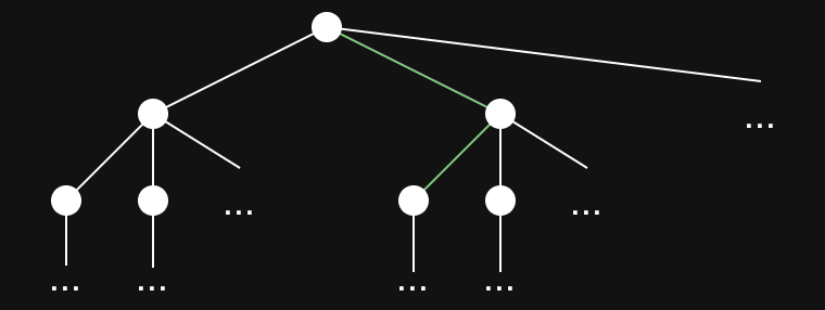
We define the ordering on this domain for any \(\rho_1, \rho_2 \in \mathrm{Dom}\) as follows:

\[\rho_1 \sqsubseteq \rho_2 \Leftrightarrow \forall M \in \Lambda(\emptyset) (\rho_1(M) \subseteq \rho_2(M)).\]

This ordering is a partial ordering since it inherits a partial ordering point-wise from the subset relation.

We define the least element (bottom element) as the following constant map:

\[\bot(M) = \emptyset.\]

We define the supremum of an \(\omega\)-chain \((\rho_n)_{n \in \mathbb{N}}\) as follows:

\[\left(\bigsqcup_{n \in \mathbb{N}}\rho_n\right)(M) = \bigcup_{n \in \mathbb{N}}\rho_n(M).\]

In fact, as an accidental side effect of this construction, the domain is even a complete lattice (i.e., it has all meets as well). However, since meets are operationally meaningless and since we make no use of them, we eventually abstract this construction from a complete lattice to a pointed, \(\omega\)-complete partial order.

We define the concatenation of a head index \(n \in \mathbb{N}\) with a tail path \(s \in \mathbb{N}^*\) of length \(k\) as a path \(n \cdot s\) of length \(k+1\) as follows:

\[(n \cdot s)_i = \begin{cases}n & \text{if } i = 0 \\ s_{i-1} & \text{if } i \ge 1\end{cases}.\]

Note that, when \(s = \varepsilon\), this constructs a singleton sequence with \((n \cdot \varepsilon)_0 = n\).

The Continuous Operator

We next define a continuous operator that elaborates trees one level at a time (i.e., it constructs them iteratively).

Call-by-Name

The call-by-name variant of this operator is a map \(\Phi_{\mathrm{n}} : \mathrm{Dom} \rightarrow \mathrm{Dom}\) defined as follows:

\[\Phi_{\mathrm{n}}(\rho)(M) = \{ \varepsilon \} \cup \{n \cdot s \mid n \in \mathbb{N} \land \exists x \in \mathcal{V}\exists M' \in \Lambda(M \Downarrow_{\mathrm{n}} (\lambda x . M') \land s \in \rho(M'[t^{\mathrm{n}}_n/x])\}.\]

When used with the Kleene Fixed Point iteration procedure, this operator builds sets of paths by appending a head index to an increasingly long tail path, which is tantamount to building a tree one level at a time.

Continuity

We establish that this operator is indeed continuous (and hence also monotone).

Theorem (Continuity). The map \(\Phi_{\mathrm{n}}\) is continuous.

Proof. Our goal is to show that

\[\Phi_{\mathrm{n}}\left(\bigsqcup_{n \in \mathbb{N}}\rho_n\right) = \bigsqcup_{n \in \mathbb{N}}\Phi_{\mathrm{n}}(\rho_n),\]

i.e., that, for all \(M \in \Lambda(\emptyset)\),

\[\Phi_{\mathrm{n}}\left(\bigsqcup_{n \in \mathbb{N}}\rho_n\right)(M) = \left(\bigsqcup_{n \in \mathbb{N}}\Phi_{\mathrm{n}}(\rho_n)\right)(M),\]

which means that

\[\Phi_{\mathrm{n}}\left(\bigsqcup_{n \in \mathbb{N}}\rho_n\right)(M) = \bigcup_{n \in \mathbb{N}}\Phi_{\mathrm{n}}(\rho_n)(M).\]

Part 1: \(\Phi_{\mathrm{n}}\left(\bigsqcup_{n \in \mathbb{N}}\rho_n\right)(M) \subseteq \bigcup_{n \in \mathbb{N}}\Phi_{\mathrm{n}}(\rho_n)(M)\). Suppose \(\sigma \in \Phi_{\mathrm{n}}\left(\bigsqcup_{k \in \mathbb{N}}\rho_k\right)(M)\). Expanding the definition, this means that

\[\sigma \in \Phi_{\mathrm{n}}(\rho)(M) = \{ \varepsilon \} \cup \{n \cdot s \mid n \in \mathbb{N} \land \exists x \in \mathcal{V}\exists M' \in \Lambda(\emptyset)(M \Downarrow_{\mathrm{n}} (\lambda x . M') \land s \in \left(\bigsqcup_{k \in \mathbb{N}}\rho_k\right)(M'[t^{\mathrm{n}}_n/x])\}.\]

Case 1: \((\sigma = \varepsilon)\). Since \(\varepsilon \in \Phi_{\mathrm{n}}(\rho_n)(M)\) for every \(n \in \mathbb{N}\), it follows that \(\sigma \in \bigcup_{k \in \mathbb{N}}\Phi_{\mathrm{n}}(\rho_k)(M)\).

Case 2: \((\sigma \in \{n \cdot s \mid n \in \mathbb{N} \land \exists x \in \mathcal{V}\exists M' \in \Lambda(M \Downarrow_{\mathrm{n}} (\lambda x . M') \land s \in \left(\bigsqcup_{n \in \mathbb{N}}\rho_n\right)(M'[t^{\mathrm{n}}_n/x])\})\). Then, there exists a natural numbers \(n \in \mathbb{N}\), a path \(s \in \mathbb{N}^*\), a variable \(x \in \mathcal{V}\), and a term \(M' \in \Lambda\) such that \(\sigma = n \cdot s\), \(M \Downarrow_{\mathrm{n}} (\lambda x . M')\), and \(s \in \left(\bigsqcup_{k \in \mathbb{N}}\rho_k\right)(M'[t^{\mathrm{n}}_n/x])\). This means that \(s \in \bigcup_{k \in \mathbb{N}}\rho_k(M'[t^{\mathrm{n}}_n/x])\) and thus there exists some \(k \in \mathbb{N}\) such that \(s \in \rho_k(M'[t^{\mathrm{n}}_n/x])\). This implies that \(\sigma = n \cdot s \in \Phi_{\mathrm{n}}(\rho_k)(M)\) and hence that \(\sigma \in \bigcup_{k \in \mathbb{N}}\Phi_{\mathrm{n}}(\rho_k)(M)\).

Part 2: \((\bigcup_{n \in \mathbb{N}}\Phi_{\mathrm{n}}(\rho_n)(M) \subseteq \Phi_{\mathrm{n}}\left(\bigsqcup_{n \in \mathbb{N}}\rho_n\right)(M))\). Suppose \(\sigma \in \bigcup_{n \in \mathbb{N}}\Phi_{\mathrm{n}}(\rho_n)(M)\). Then there exists an index \(k \in \mathbb{N}\) such that \(\sigma \in \Phi_{\mathrm{k}}(\rho_k)(M)\).

Case 1: \((\sigma = \varepsilon)\). Since \(\varepsilon \in \Phi_{\mathrm{n}}(\rho_n)(M)\) for every \(n \in \mathbb{N}\), it follows that \(\sigma \in \Phi_{\mathrm{n}}\left(\bigsqcup_{n \in \mathbb{N}}\rho_n\right)(M)\).

Case 2: \((\sigma \in \{n \cdot s \mid n \in \mathbb{N} \land \exists x \in \mathcal{V}\exists M' \in \Lambda(M \Downarrow_{\mathrm{n}} (\lambda x . M') \land s \in \rho(M'[t^{\mathrm{n}}_n/x])\})\). Then there exists a natural number \(n \in \mathbb{N}\), a path \(s \in \mathbb{N}^*\), a variable \(x \in \mathcal{V}\), and a term \(M' \in \Lambda\) such that \(\sigma = n \cdot s\), \(M \Downarrow_{\mathrm{n}} (\lambda x . M')\), and \(s \in \rho_k(M'[t^{\mathrm{n}}_n/x])\). Since \(\bigsqcup_{k \in \mathbb{N}}\rho_k\) is a supremum of the chain \((\rho_k)_{k \in \mathbb{N}}\), it follows that \(\rho_k(M'[t^{\mathrm{n}}_n/x]) \subseteq \left(\bigsqcup_{k \in \mathbb{N}}\rho_k\right)(M'[t^{\mathrm{n}}_n/x])\) and hence \(s \in \left(\bigsqcup_{k \in \mathbb{N}}\rho_k\right)(M'[t^{\mathrm{n}}_n/x])\). As a result, \(\sigma = n \cdot s \in \Phi_{\mathrm{n}}\left(\bigsqcup_{k \in \mathbb{N}}\rho_k\right)(M)\).

\(\square\)

Call-by-Value

The call-by-value variant of this operator is a map \(\Phi_{\mathrm{v}} : \mathrm{Dom} \rightarrow \mathrm{Dom}\) defined as follows:

\[\Phi_{\mathrm{v}}(\rho)(M) = \{ \varepsilon \} \cup \{n \cdot s \mid n \in \mathbb{N} \land \exists x \in \mathcal{V}\exists M' \in \Lambda(M \Downarrow_{\mathrm{n}} (\lambda x . M') \land s \in \rho(M'[t^{\mathrm{v}}_n/x])\}.\]

When used with the Kleene Fixed Point iteration procedure, this operator builds sets of paths by appending a head index to an increasingly long tail path, which is tantamount to building a tree one level at a time.

Continuity

We establish that this operator is indeed continuous (and hence also monotone).

Theorem (Continuity). The map \(\Phi_{\mathrm{v}}\) is continuous.

Proof. Nearly identical to the call-by-name case. \(\square\)

Fixed Points

The Kleene Fixed Point Theorem indicates that, in a CPO, every continuous operator \(f\) on the CPO has a least fixed point given by

\[\mu f = \bigsqcup_{n \in \mathbb{N}}f^n(\bot).\]

Thus, we compute the least fixed points

\[\mu \Phi_{\mathrm{n}} = \bigsqcup_{n \in \mathbb{N}} \Phi_{\mathrm{n}}^n(\bot)\]

and

\[\mu \Phi_{\mathrm{v}} = \bigsqcup_{n \in \mathbb{N}} \Phi_{\mathrm{v}}^n(\bot).\]

These fixed points completely characterize the behavior (i.e., coinductive unfolding) of closed lambda terms.

Example

Let's consider an example of this iterative unfolding for a given closed term \(M\).

At iteration \(0\), we compute

\[\Phi_{\mathrm{n}}^0(\bot)(M) = \bot(M) = \emptyset.\]

At iteration \(1\), we compute

\begin{align*}\Phi_{\mathrm{n}}^1(\bot)(M) &= \{ \varepsilon \} \cup \{n \cdot s \mid n \in \mathbb{N} \land \exists x \in \mathcal{V}\exists M' \in \Lambda(M \Downarrow_{\mathrm{n}} (\lambda x . M') \land s \in \Phi_{\mathrm{n}}^0(M'[t^{\mathrm{n}}_n/x])\} \\&= \{\varepsilon\}.\end{align*}

At iteration \(2\), we compute

\begin{align*}\Phi_{\mathrm{n}}^2(\bot)(M) &= \{ \varepsilon \} \cup \{n \cdot s \mid n \in \mathbb{N} \land \exists x \in \mathcal{V}\exists M' \in \Lambda(M \Downarrow_{\mathrm{n}} (\lambda x . M') \land s \in \Phi_{\mathrm{n}}^1(\bot)(M'[t^{\mathrm{n}}_n/x])\} \\&= \{\varepsilon\} \cup \begin{cases} \emptyset & \text{if } M \Uparrow_{\mathrm{n}} \\ \mathbb{N}^1 & \text{otherwise} \end{cases}.\end{align*}

\begin{align*}\Phi_{\mathrm{n}}(\bot)^3(M) &= \{ \varepsilon \} \cup \{n \cdot s \mid n \in \mathbb{N} \land \exists x \in \mathcal{V}\exists M' \in \Lambda(M \Downarrow_{\mathrm{n}} (\lambda x . M') \land s \in \Phi_{\mathrm{n}}(\bot)^2(M'[t^{\mathrm{n}}_n/x])\} \\&= \{\varepsilon\} \cup \begin{cases}\emptyset & \text{if } M \Uparrow_{\mathrm{n}} \\ \mathbb{N}^1 \cup \{n_1 \cdot n_2 \cdot \varepsilon \mid M'[t^{\mathrm{n}}_{n_1}/x] \Downarrow_{\mathrm{n}} \land n_2 \in \mathbb{N}\} & \text{otherwise} \end{cases}.\end{align*}

Thus, the following pattern emerges: at iteration \(k+1\), all convergent paths of length \(k\) rooted at \(M\) have been computed (i.e., \(k\) levels of the tree have been elaborated). Whenever a term diverges, the respective path terminates.

Applicative Bisimilarity Implies Tree Equality

Next, we will show that applicative bisimilarity implies tree equality.

Call-by-Name

In this section, we consider the call-by-name case.

Theorem. For any pair of closed lambda terms \(M, N \in \Lambda(\emptyset)\), if \(M \sim_{\mathrm{n}} N\), then \(\mu \Phi_{\mathrm{n}}(M) = \mu \Phi_{\mathrm{n}}(N)\).

Proof. Recall that

\[\mu \Phi_{\mathrm{n}} = \bigsqcup_{n \in \mathbb{N}} \Phi_{\mathrm{n}}^n(\bot).\]

We therefore proceed by induction on the iteration rank \(n\); we will show that, for all \(n \in \mathbb{N}\), \(\Phi^n_{\mathrm{n}}(\bot)(M) = \Phi^n_{\mathrm{n}}(\bot)(N)\).

Base Case: \((n=0)\). By definition,

\begin{align*}\Phi^0_{\mathrm{n}}(\bot)(M) &= \bot(M) \\&= \emptyset \\&= \bot(N) \\&= \Phi^0_{\mathrm{n}}(\bot)(N).\end{align*}

Induction Step: Assume for some fixed \(n \in \mathbb{N}\) that, for any pair of terms \(P, Q \in \Lambda(\emptyset)\), if \(P \sim_{\mathrm{n}} Q\), then \(\Phi^n_{\mathrm{n}}(\bot)(P) = \Phi^n_{\mathrm{n}}(\bot)(Q)\).

Suppose \(M \sim_{\mathrm{n}} N\). By definition,

\[\Phi_{\mathrm{n}}^{n+1}(\bot)(M) = \{ \varepsilon \} \cup \{k \cdot s \mid k \in \mathbb{N} \land \exists x \in \mathcal{V} \exists M' \in \Lambda (M \Downarrow_{\mathrm{n}} (\lambda x . M') \land s \in \Phi_{\mathrm{n}}^n(\bot)(M'[t_n^{\mathrm{n}}/x]))\}.\]

Since \(M \sim_{\mathrm{n}} N\), either both terms diverge or both converge.

Case 1: if both terms diverge, then \(\Phi_{\mathrm{n}}^{n+1}(\bot)(M) = \{\varepsilon\} = \Phi_{\mathrm{n}}^{n+1}(\bot)(N) \).

Case 2: if both terms converge, then, for any test index \(k \in \mathbb{N}\), by definition of applicative bisimilarity, \(M'[t_n^{\mathrm{n}}/x] \sim_{\mathrm{n}} N'[t_n^{\mathrm{n}}/x]\), which, by the inductive hypothesis, means that

\[\Phi_{\mathrm{n}}^n(\bot)(M'[t_n^{\mathrm{n}}/x]) = \Phi_{\mathrm{n}}^n(\bot)(N'[t_n^{\mathrm{n}}/x]).\]

This then implies that the set of paths \(k \cdot s\) is identical for \(s \in \Phi_{\mathrm{n}}^n(\bot)(M'[t_n^{\mathrm{n}}/x])\) and \(s \in \Phi_{\mathrm{n}}^n(\bot)(N'[t_n^{\mathrm{n}}/x])\), so

\[\Phi_{\mathrm{n}}^{n+1}(\bot)(M) = \Phi_{\mathrm{n}}^{n+1}(\bot)(N).\]

Thus, by induction, it follows for all \(n \in \mathbb{N}\) that

\[\Phi_{\mathrm{n}}^n(\bot)(M) = \Phi_{\mathrm{n}}^n(\bot)(N).\]

It then follows that

\begin{align*}\mu \Phi_{\mathrm{n}}(M) &= \bigcup_{n \in \mathbb{N}} \Phi_{\mathrm{n}}(\bot)(M)\\&= \bigcup_{n \in \mathbb{N}} \Phi_{\mathrm{n}}(\bot)(N) \\&= \mu \Phi_{\mathrm{n}}(N).\end{align*}

\(\square\)

Call-by-Value

In this section, we consider the call-by-value case.

Theorem. For any pair of closed lambda terms \(M, N \in \Lambda(\emptyset)\), if \(M \sim_{\mathrm{n}} N\), then \(\mu \Phi_{\mathrm{v}}(M) = \mu \Phi_{\mathrm{n}}(N)\).

Proof. The proof is virtually identical to the call-by-name case. \(\square\)

Tree Equality Implies Applicative Bisimilarity

Next, we will show that tree equality implies applicative bisimilarity.

Call-by-Name

We consider the call-by-name case first.

Theorem. For any pair of closed lambda terms \(M, N \in \Lambda(\emptyset)\), if \(\mu\Phi_{\mathrm{n}}(M) = \mu\Phi_{\mathrm{n}}(N)\), then \(M \sim_{\mathrm{n}} N\).

Proof. We define a relation \(R \subseteq \Lambda(\emptyset) \times \Lambda(\emptyset)\) as follows:

\[R = \{(M,N) \in \Lambda(\emptyset) \times \Lambda(\emptyset) \mid \mu\Phi_{\mathrm{n}}(M) = \mu\Phi_{\mathrm{n}}(N)\}.\]

We will show that this relation is an applicative bisimulation, thus implying that it is contained in applicative bisimilarity, which is the largest applicative bisimulation.

Suppose \(M \mathrel{R} N\).

Part 1: Convergence

Suppose \(M \Downarrow_{\mathrm{n}}\). Then, since \(\varepsilon \in \Phi_{\mathrm{n}}(\mu \Phi_{\mathrm{n}})(M)\) and \(\mu \Phi_{\mathrm{n}} = \Phi_{\mathrm{n}}(\mu \Phi_{\mathrm{n}})\), it follows that \(\varepsilon \in \mu \Phi_{\mathrm{n}}(M)\). Then, since \(M \Downarrow_{\mathrm{n}}\), this implies that \(n \cdot \varepsilon \in \Phi_{\mathrm{n}}(\mu \Phi_{\mathrm{n}})(M)\) for all \(n \in \mathbb{N}\), and hence \(n \cdot \varepsilon \in \mu \Phi_{\mathrm{n}}(M)\). Since \(M \mathrel{R} N\), it follows that \(\mu\Phi_{\mathrm{n}}(M) = \mu\Phi_{\mathrm{n}}(N)\) and hence \(n \cdot \varepsilon \in \mu \Phi_{\mathrm{n}}(N)\) and thus \(n \cdot \varepsilon \in \Phi_{\mathrm{n}}(\mu \Phi_{\mathrm{n}})(N)\), which implies that \(N \Downarrow_{\mathrm{n}}\).

The converse argument is entirely symmetric. Thus, \(M \Downarrow_{\mathrm{n}}\) if and only if \(N \Downarrow_{\mathrm{n}}\).

Part 2: Application

Suppose \(M \Downarrow_{\mathrm{n}} (\lambda x . M')\) and \(N \Downarrow_{\mathrm{n}} (\lambda x . N')\). Let \(k \in \mathbb{N}\) be any test index. Let \(s \in \mathbb{N}^*\) be any trace. Then \(s \in \mu \Phi_{\mathrm{n}}(M'[t^{\mathrm{n}}_k])\) if and only if \(k \cdot s \in \Phi_{\mathrm{n}}(\mu \Phi_{\mathrm{n}})(M) = \mu \Phi_{\mathrm{n}}(M)\). Since \(M \mathrel{R} N\), it follows that \(\mu\Phi_{\mathrm{n}}(M) = \mu\Phi_{\mathrm{n}}(N)\) and hence \(k \cdot s \in \mu \Phi_{\mathrm{n}}(M)\) if and only if \(k \cdot s \in \mu \Phi_{\mathrm{n}}(N)\). Furthermore, \(s \in \mu \Phi_{\mathrm{n}}(N'[t^{\mathrm{n}}_k])\) if and only if \(k \cdot s \in \Phi_{\mathrm{n}}(\mu \Phi_{\mathrm{n}})(N) = \mu \Phi_{\mathrm{n}}(N)\). From this, we conclude that \(k \cdot s \in \mu \Phi_{\mathrm{n}}(M'[t^{\mathrm{n}}_k])\) if and only if \(k \cdot s \in \mu \Phi_{\mathrm{n}}(N'[t^{\mathrm{n}}_k])\), i.e., that \(\mu \Phi_{\mathrm{n}}(M'[t^{\mathrm{n}}_k]) = \mu \Phi_{\mathrm{n}}(N'[t^{\mathrm{n}}_k])\) and hence \(M'[t^{\mathrm{n}}_k] \mathrel{R} N'[t^{\mathrm{n}}_k]\).

Thus, \(R\) is an applicative bisimulation, and therefore \(R \subseteq \sim_{\mathrm{n}}\), i.e., if \(\mu\Phi_{\mathrm{n}}(M) = \mu\Phi_{\mathrm{n}}(N)\), then \(M \sim_{\mathrm{n}} N\). \(\square\)

Equivalence of Applicative Bisimilarity and Tree Equality

We have thus shown the following:

\[M \sim_{\mathrm{n}} N \Leftrightarrow \mu\Phi_{\mathrm{n}}(M) = \mu\Phi_{\mathrm{n}}(N).\]

Conclusion

We described a concrete CPO \(\mathrm{Dom}\) which represents partial unfoldings of closed lambda term traces. In such a design, applicative bisimilarity coincides with trace tree equality, and hence such trees are extensional representations of lambda term behavior. Abstracting away from this, we can use CPOs generally for denotational semantics.

This explains the somewhat vague intuition that the elements of a CPO domain represent "partial information" about a lambda term; concretely, we have shown that we may interpret this partial information as a rank-\(n\) trace tree. The ordering is simply tree inclusion. The supremum represents the "complete information", i.e., an infinitary trace tree. This supremum can be computed using the Kleene fixed point iteration method, which gives us a way to model the coinductive unfolding of a lambda term trace.